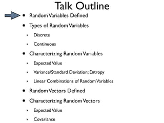
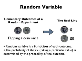
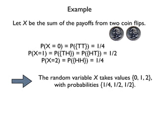
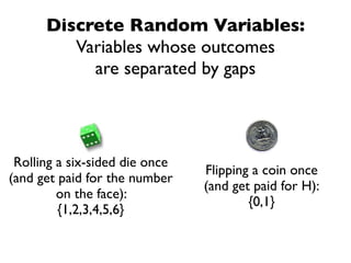
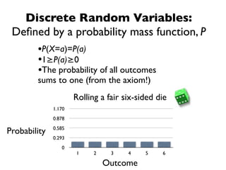
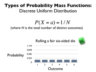
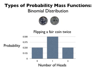
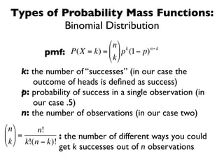
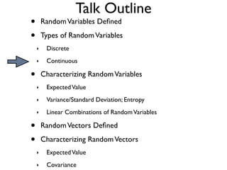
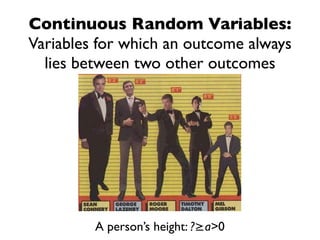
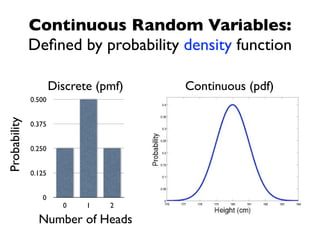
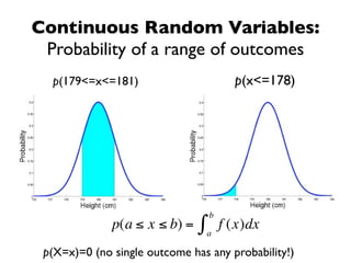
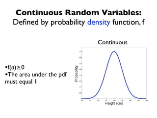
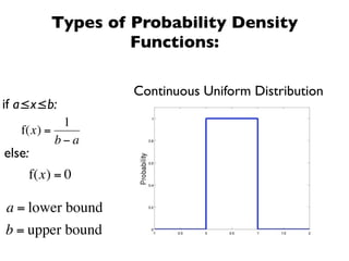
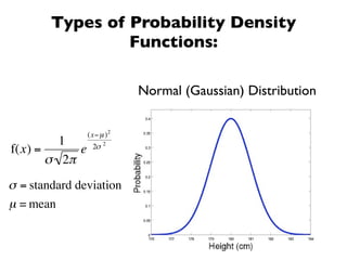
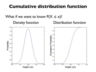
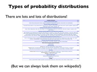
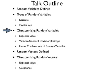
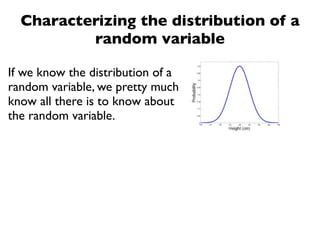
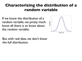
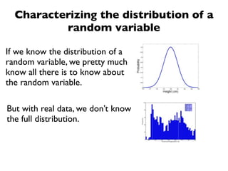
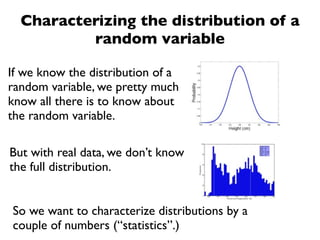
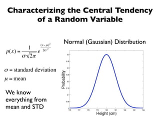
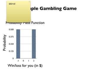
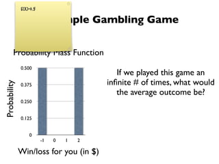
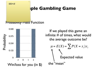
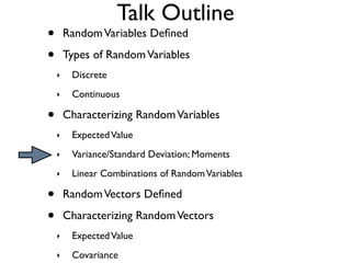
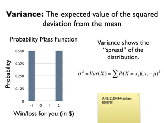
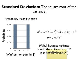
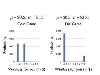
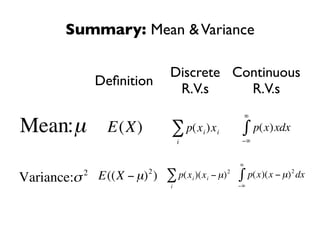
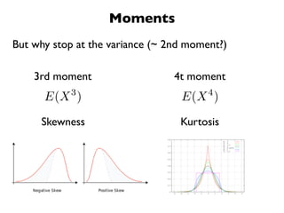
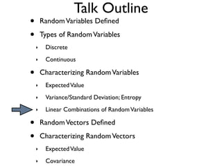
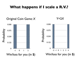
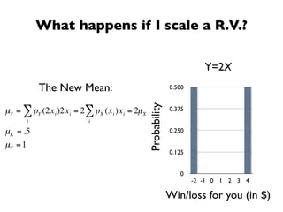
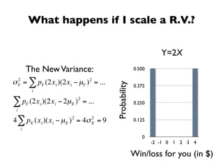
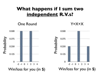
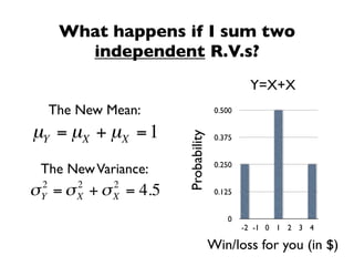
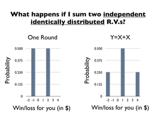
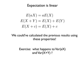
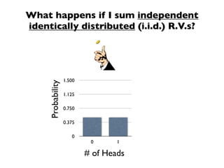
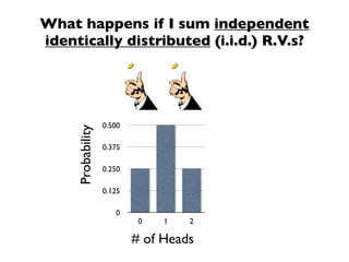
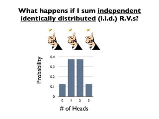
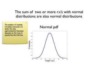
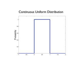
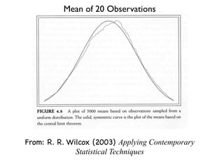
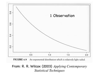
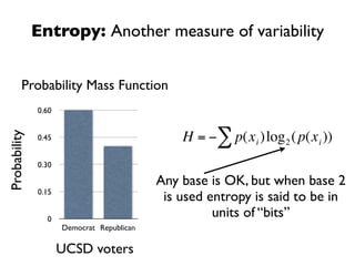
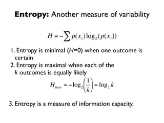
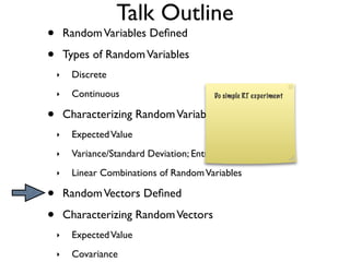
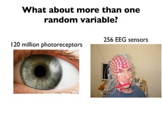
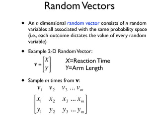
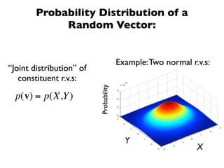
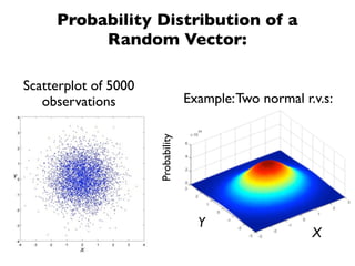
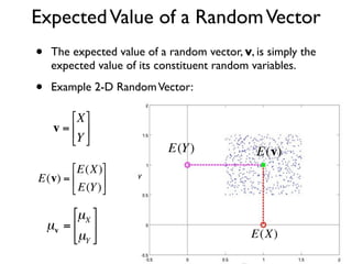
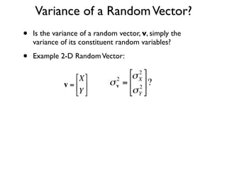
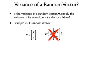
Random Variables

Random Variables/Vectors
Tomoki Tsuchida
Computational & Cognitive Neuroscience Lab
Department of Cognitive Science
University of California, San Diego

Talk Outline
• Random Variables Deﬁned

• Types of Random Variables
‣ Discrete
‣ Continuous

• Characterizing Random Variables
‣ Expected Value
‣ Variance/Standard Deviation; Entropy
‣ Linear Combinations of Random Variables

• Random Vectors Deﬁned

• Characterizing Random Vectors
‣ Expected Value
‣ Covariance

Random Variable

Elementary Outcomes of a
The Real Line
Random Experiment

=$1

Flipping a coin once =$0

• Random variable is a function of each outcome.
• The probability of the r.v. (taking a particular value) is
determined by the probability of the outcome.

Example
Let X be the sum of the payoffs from two coin ﬂips.

P(X = 0) = P({TT}) = 1/4
P(X=1) = P({TH}) = P({HT}) = 1/2
P(X=2) = P({HH}) = 1/4

The random variable X takes values {0, 1, 2},
with probabilities {1/4, 1/2, 1/2}.

Discrete Random Variables:
Variables whose outcomes
are separated by gaps

Rolling a six-sided die once
Flipping a coin once
(and get paid for the number
(and get paid for H):
on the face):
{0,1}
{1,2,3,4,5,6}

Discrete Random Variables:
Deﬁned by a probability mass function, P
•P(X=a)=P(a)
•1≥P(a)≥0
•The probability of all outcomes
sums to one (from the axiom!)
Rolling a fair six-sided die
1.170
0.878
0.585
Probability
0.293
0
1 2 3 4 5 6

Outcome

Types of Probability Mass Functions:
Discrete Uniform Distribution

P(X = a) = 1 / N
(where N is the total number of distinct outcomes)

Rolling a fair six-sided die
€ 1.170
0.878
0.585
Probability
0.293
0
1 2 3 4 5 6

Outcome

Binomial Distribution

Flipping a fair coin twice
0.500

0.375
Probability 0.250

0.125

0
0 1 2

Number of Heads

Binomial Distribution
⎛ n ⎞ k n−k
pmf: P(X = k) = ⎜ ⎟ p (1− p)
⎝ k ⎠
k: the number of “successes” (in our case the
outcome of heads is deﬁned as success)
p: probability of success in a single observation (in
€
our case .5)
n: the number of observations (in our case two)
⎛ n ⎞ n!
⎜ ⎟ = : the number of different ways you could
⎝ k ⎠ k!(n − k)!
get k successes out of n observations

Continuous Random Variables:
Variables for which an outcome always
lies between two other outcomes

A person’s height: ?≥a>0

Deﬁned by probability density function

Discrete (pmf) Continuous (pdf)
0.500
Probability

0.375

0.250

0.125

0
0 1 2

Number of Heads

Probability of a range of outcomes
p(179<=x<=181) p(x<=178)

b
p(a ≤ x ≤ b) = ∫ a
f (x)dx
p(X=x)=0 (no single outcome has any probability!)

Deﬁned by probability density function, f

Continuous

•f(a)≥0
•The area under the pdf
must equal 1

Types of Probability Density
Functions:

Continuous Uniform Distribution
if a≤x≤b:
1
f(x) =
b−a
else:
f(x) = 0

a = lower bound
b = upper bound

Types of Probability Density
Functions:

Normal (Gaussian) Distribution

(x− µ )2
1 2
f(x) = e 2σ
σ 2π
σ = standard deviation
µ = mean

Cumulative distribution function

What if we want to know P(X ≤ x)?
Density function Distribution function

Types of probability distributions

There are lots and lots of distributions!

(But we can always look them on wikipedia!)

Characterizing the distribution of a
random variable

If we know the distribution of a
random variable, we pretty much
know all there is to know about
the random variable.

random variable


But with real data, we don’t know
the full distribution.

random variable


But with real data, we don’t know
the full distribution.

So we want to characterize distributions by a
couple of numbers (“statistics”.)

Characterizing the Central Tendency
of a Random Variable

(x− µ )2
Normal (Gaussian) Distribution
1 2
p(x) = e 2σ
σ 2π

σ = standard deviation
µ = mean

We know
everything from
mean and STD

A Simple Gambling Game

1. Flip a fair coin
2. Possible outcomes:

I give you $2
P(X=2)=1/2
P(X=-1)=1/2
You give me $1

E(X)=$.5


Probability Mass Function
0.500
Probability

0.375

0.250

0.125

0
-1 0 1 2

Win/loss for you (in $)

E(X)=$.5


0.500
If we played this game an
inﬁnite # of times, what would
Probability

0.375
the average outcome be?
0.250

0.125

0
-1 0 1 2


E(X)=$.5


0.500
If we played this game an
inﬁnite # of times, what would
Probability

0.375
the average outcome be?
0.250
µ = E(X) = ∑ P(X = x i )x i
0.125

0 Expected value
-1 0 1 2
€ the “mean”

Another Gambling Game
1. Roll a fair six-sided die
2. Possible outcomes:
Die Payoff
1 $8
2 -$1
3 -$1
4 -$1
5 -$1
6 -$1

Another Gambling Game

0.900

What’s the mean outcome
Probability

0.675
of this game?
0.450
µ = E(X) = ∑ P(X = x i )x i
0.225

0
-1 0 1 2 3 4 5 6 7 8
€
Win/loss for you (in $) E(X)=$.5

Why should you prefer the coin
game?
Coin Game Die Game
0.850 0.900
Probability

Probability
0.638 0.675

0.425 0.450

0.213 0.225

0 0
-1 0 1 2 3 4 5 6 7 8 -1 0 1 2 3 4 5 6 7 8

Win/loss for you (in $) Win/loss for you (in $)

Talk Outline

‣ Discrete
‣ Continuous

‣ Expected Value
‣ Variance/Standard Deviation; Moments


‣ Expected Value
‣ Covariance

Characterizing the Variability of a
Random Variable
Coin Game Die Game
0.850 0.900
Probability

Probability
0.638 0.675

0.425 0.450

0.213 0.225

0 0
-1 0 1 2 3 4 5 6 7 8 -1 0 1 2 3 4 5 6 7 8


Variance: The expected value of the squared
deviation from the mean
Probability Mass Function Variance shows the
0.500 “spread” of the
distribution.
Probability

0.375

0.250
σ 2 = Var(X) = ∑ P(X = x i )(x i − µ) 2

0.125

ANS: 2.25=9/4 dollars
0 € squared
-1 0 1 2


Standard Deviation: The square root of the
variance
0.500
Probability

0.375
σ 2 = Var(X) = ∑ P(X = x i )(x i − µ) 2
0.250
σ = Var(X)
0.125
€ (Why? Because variance
0
-1 0 1 2 €was in the units of X2. STD
is in the same unit X.)
ANS: 1.5 dollars

µ = $0.5, σ = $1.5 µ = $0.5, σ ≈ $3.35
Coin Game Die Game
0.850 0.900

€
Probability

Probability
0.638 0.675

0.425 0.450

0.213 0.225

0 0
-1 0 1 2 3 4 5 6 7 8 -1 0 1 2 3 4 5 6 7 8


Summary: Mean & Variance

Discrete Continuous
Deﬁnition
R.V.s R.V.s
∞

Mean:µ E(X) ∑ p(x )x i i ∫ p(x)xdx
i −∞

∞
2 2
Variance:σ 2
E((X − µ) ) ∑ p(x i )(x i − µ) 2 ∫ p(x)(x − µ) dx
€ i € −∞

€
€ €
€

Moments
But why stop at the variance (~ 2nd moment?)

3rd moment 4t moment
E(X 3 ) E(X 4 )
Skewness Kurtosis

What happens if I scale a R.V.?

Original Coin Game: X Y=2X
0.500 0.500

Probability
Probability

0.375 0.375

0.250 0.250

0.125 0.125

0 0
-1 0 1 2 -2 -1 0 1 2 3 4



Y=2X
The New Mean: 0.500

Probability
µY = ∑ pY (2x i )2x i = 2∑ pX (x i )x i = 2µX 0.375
i i

µX = .5 0.250

µY = 1
0.125

0
-2 -1 0 1 2 3 4



Y=2X
The New Variance: 0.500

σ Y = ∑ pY (2x i )(2x i − µY ) 2 = ...
2

Probability
0.375
i

∑ pY (2x i )(2x i − 2µX ) 2 = ... 0.250
i

4 ∑ pX (x i )(x i − µX ) 2 = 4σ X = 9
2
0.125
i
0
-2 -1 0 1 2 3 4


What happens if I sum two
independent R.V.s?
One Round Y=X+X
0.500 0.500
Probability

Probability
0.375 0.375

0.250 0.250

0.125 0.125

0 0
-2 -1 0 1 2 3 4 -2 -1 0 1 2 3 4


What happens if I sum two
independent R.V.s?
Y=X+X
The New Mean: 0.500

µY = µX + µX = 1

Probability
0.375

0.250
The New Variance:
2 2 2
σ = σ + σ = 4.5
Y X X 0.125

0
-2 -1 0 1 2 3 4


What happens if I sum two independent
identically distributed R.V.s?

One Round Y=X+X
0.500 0.500
Probability

Probability
0.375 0.375

0.250 0.250

0.125 0.125

0 0
-2 -1 0 1 2 3 4 -2 -1 0 1 2 3 4


Expectation is linear

E(aX) = aE(X)
E(X + Y ) = E(X) + E(Y )
E(X + c) = E(X) + c

We could’ve calculated the previous results using
these properties!

Exercise: what happens to Var(aX)
and Var(X+Y) ?

What happens if I sum independent
identically distributed (i.i.d.) R.V.s?

1.500
Probability

1.125

0.750

0.375

0
0 1

# of Heads


0.500
Probability

0.375

0.250

0.125

0
0 1 2

# of Heads


0.4
Probability

0.3

0.2

0.1

0
0 1 2 3

# of Heads


0.4
Probability

0.3

0.2

0.1

0
0 1 2 3 4

# of Heads


What’s happening to the
Mean of 75 ﬂips
pmf?

Ans: it’s looking more
and more Gaussian


Mean of 150 ﬂips

Central Limit Theorem:
The sum of i.i.d. random variables is approximately
normally distributed when the number of random
This is one reason why
variables is large.
Gaussian variables are
popularly assumed when
doing statistical analysis
Normal pdf
or modeling. Another Mean of 150 ﬂips
reason is that it’s
mathematically simpler

from: Oxford Dictionary of Statistics

The sum of two or more r.v.’s with normal
distributions are also normal distributions

The number of random
variables necessary to
make the sum
Normal pdf
approximately Gaussian
depends on the type of
population distribution

Continuous Uniform Distribution

Mean of 20 Observations

From: R. R. Wilcox (2003) Applying Contemporary
Statistical Techniques

1 Observation


mean of 25 samples


Wilcox says you need
100 samples from this
distribution to get a
decent approximation

mean of 50 samples


Entropy: Another measure of variability

0.60

H = −∑ p(x i )log 2 ( p(x i ))
Probability

0.45

0.30

Any base is OK, but when base 2
0.15
is used entropy is said to be in
€ units of “bits”
0
Democrat Republican

UCSD voters

Entropy: Another measure of variability

H = −∑ p(x i )log 2 ( p(x i ))

1. Entropy is minimal (H=0) when one outcome is
certain
2. Entropy is maximal when each of the
€
k outcomes is equally likely
⎛ 1 ⎞
H max = −log 2 ⎜ ⎟ = log 2 k
⎝ k ⎠

3. Entropy is a measure of information capacity.

€

Talk Outline

‣ Discrete
‣ Continuous Do simple RT experiment

‣ Expected Value
‣ Variance/Standard Deviation; Entropy


‣ Expected Value
‣ Covariance

What about more than one
random variable?

256 EEG sensors
120 million photoreceptors

Random Vectors
• An n dimensional random vector consists of n random
variables all associated with the same probability space
(i.e., each outcome dictates the value of every random
variable)

• Example 2-D Random Vector:
⎡X ⎤ X=Reaction Time
v = ⎢ ⎥
⎣Y ⎦ Y=Arm Length

• Sample m times from v:
v1 v 2 v 3 ... v m
€
⎡x1 x2 x 3 ... x m ⎤
⎢ ⎥
⎣y1 y2 y 3 ... y m ⎦

Probability Distribution of a
Random Vector:

Example: Two normal r.v.s:
“Joint distribution” of
constituent r.v.s:

Probability
p(v) = p(X,Y )

Y
X

Probability Distribution of a
Random Vector:

Scatterplot of 5000
observations Example: Two normal r.v.s:

Probability

Y
X

What will the scatterplot of
our data look like?
A: B:

C: D:

Expected Value of a Random Vector
• The expected value of a random vector, v, is simply the
expected value of its constituent random variables.


⎡X ⎤
v = ⎢ ⎥
⎣Y ⎦
E(Y ) E(v)
⎡ E(X)⎤
E(v) = ⎢ ⎥
⎣ E(Y ) ⎦
€
€ €
⎡µX ⎤
µv = ⎢ ⎥
⎣µY ⎦ E(X)

Variance of a Random Vector?
• Is the variance of a random vector, v, simply the
variance of its constituent random variables?


⎡X ⎤ 2
⎡σ X ⎤
2

v = ⎢ ⎥ σ v = ⎢ 2 ⎥ ?
⎣Y ⎦ ⎣σ Y ⎦

€
€

Variance of a Random Vector?
• Is the variance of a random vector, v, simply the
variance of its constituent random variables?


X
⎡X ⎤ 2
⎡σ X ⎤
2

v = ⎢ ⎥ σ v = ⎢ 2 ⎥ ?
⎣Y ⎦ ⎣σ Y ⎦

€
€

X & Y all have Variance of 2

A: B:

C:

Covariance Matrix of a Random Vector
• Diagonal entries are the variance of that dimension

• Off-diagonal entries are the covariance between the
column and row dimensions
‣ Covariance between two random variables:
Cov(X,Y ) = E((X − µx )(Y − µy ))

Note: Cov(X,Y ) = Cov(Y, X)
Cov(X,Y ) = 0 if X and Y are independent
€
Cov(X,Y ) ∝ Corr(X,Y )

• Our 2-D example:
⎡X ⎤ ⎡ Var(X) Cov(Y, X)⎤
€ v = ⎢ ⎥ C = ⎢ ⎥
⎣Y ⎦ ⎣Cov(X,Y ) Var(Y ) ⎦

Which Data=which Covariance Matrix?

A: B:

C: ⎡ 2 1.5⎤
Q = ⎢ ⎥
⎣1.5 2 ⎦ ⎡2 0⎤
S = ⎢ ⎥
⎡ 2 −1.5⎤ ⎣0 2⎦
R = ⎢ ⎥
⎣−1.5 2 ⎦
€

Covariance of 0 does NOT entail
independence!!

•Recall: Cov(X,Y ) ∝ Corr(X,Y )
Cov(X,Y )
Corr(X,Y ) =
σ Xσ Y

•PMF of two dependent variables with a
covariance of 0:
€ p(X = 1,Y = 0) = .25 p(X = 0,Y = 1) = .25
p(X = −1,Y = 0) = .25 p(X = 0,Y = −1) = .25

•Special case: If two normally distributed random
variables have a covariance of 0, they ARE independent
€ €

Recommended Resources:
The Mathworld online math encyclopedia:
http://mathworld.wolfram.com/

Gonzalez & Woods: Review Chapter on Linear
Algebra, Probability, & Random Variables:
http://www.imageprocessingplace.com/root_ﬁles_V3/
tutorials.htm

Javier Movellan’s useful math facts:
http://mplab.ucsd.edu/wordpress/?page_id=75

Dana Ballard’s Natural Computation
(some good stuff)

Dayan & Abbot
Theoretical Neuroscience

Contemporary Data Analysis
Rand Wilcox, Applying Contemporary

Sheldon Ross
A First Course in Probability

Recommended Free
Stats Software

www.r-project.org

www.scipy.org

Random Variables

In this document