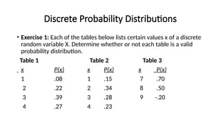
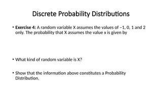
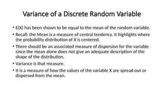
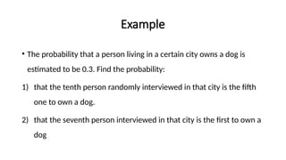
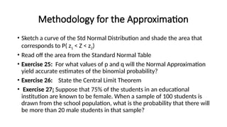
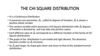
This document provides a comprehensive overview of probability distributions, focusing on discrete and continuous probability distributions, their definitions, properties, and practical applications. It includes exercises to evaluate understanding and explore various types of distributions, including uniform, Bernoulli, and binomial distributions, while emphasizing the concepts of expected value and variance. The document also discusses the mathematical formulation and characteristics of probability mass functions and density functions, ensuring that fundamental probability axioms are upheld.

![Properties of Expectation
• Let X be any discrete random variable
• If a is a constant then E(a) = a
• If a is a constant then E(aX) = a E(X)
• If b is a constant then
• E(X + b) = E(X) + b
• If a and b are constants then
• E(aX + b) = a E(X) + b
• If X and Y are two distinct random variables then
• E( X + Y) = E(X) + E(Y)
• If g(X) and h(X) are two distinct functions defined on X then
• E[g(X) + h(X)] = E[g(X)] + E[ h(X)]](https://image.slidesharecdn.com/unit2probabilitydistributions1-240922165052-d94ea943/85/Unit-2-Probability-Distributions-1-pptx-18-320.jpg)
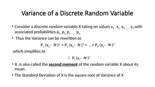


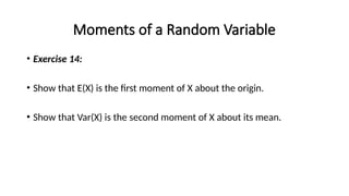
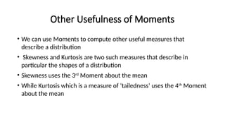
![Moments of a Random Variable
• The rth moment about the origin of a random variable X is written as
E[X r
] and is given by
E[X r
] = xr
P(x) or xr
f(x) in the discrete case
Or
• where f(x) is the probability density function of X in the continuous
case.
• This holds for r = 0,1,2,3, …….](https://image.slidesharecdn.com/unit2probabilitydistributions1-240922165052-d94ea943/85/Unit-2-Probability-Distributions-1-pptx-37-320.jpg)
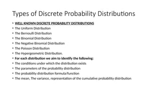
![Moments of a Random Variable
• The rth moment about the mean of a random variable X is written as
E[(X - ) r
] and is given by
E[(X - ) r
] = (x - )r
P(x) or (x - )r
f(x) in the discrete
case
Or
where f(x) is the probability density function of X in the continuous
case.
This holds for r = 0,1,2,3, …….](https://image.slidesharecdn.com/unit2probabilitydistributions1-240922165052-d94ea943/85/Unit-2-Probability-Distributions-1-pptx-38-320.jpg)
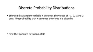
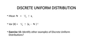
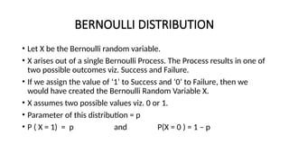
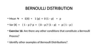
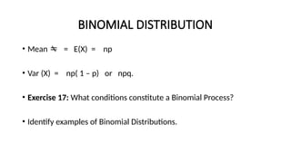
![DISCRETE UNIFORM DISTRIBUTION
• Let X be the discrete uniform random variable.
• X assumes a finite number of values, x1, x2, x3, ……xk , with equal
probabilities.
• For example: in the experiment of tossing a fair die; if we let X be the
score on the face of the die, then X assumes values of 1, 2, 3, 4, 5 & 6.
• Parameter of this distribution = k. What is k?
• P ( X = x) = 1
/k for all x in the set of values [x1, x2, x3, ……xk]
• In the example of the toss of the fair die, the probability of X
assuming any one of the six values is 1
/6.](https://image.slidesharecdn.com/unit2probabilitydistributions1-240922165052-d94ea943/85/Unit-2-Probability-Distributions-1-pptx-42-320.jpg)


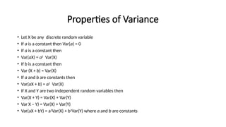
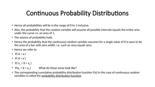
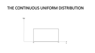
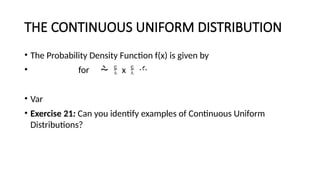
![THE CONTINUOUS UNIFORM DISTRIBUTION
• Let X be the continuous uniform random variable.
• Parameters of the distribution are and .
• X assumes values in the continuous interval of real numbers [ , .]
• The probability distribution curve is rectangular in shape.](https://image.slidesharecdn.com/unit2probabilitydistributions1-240922165052-d94ea943/85/Unit-2-Probability-Distributions-1-pptx-62-320.jpg)
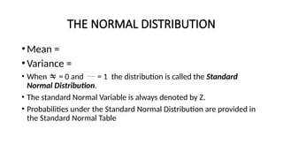
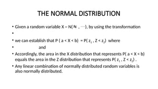
![THE NORMAL DISTRIBUTION
• Let X be the normal random variable. X assumes values in the
continuous interval of real numbers [-∞ , +∞]
• Parameters of the distribution are and .
• The probability distribution curve is bell shaped.
• The Probability Density Function f(x) is given by
•](https://image.slidesharecdn.com/unit2probabilitydistributions1-240922165052-d94ea943/85/Unit-2-Probability-Distributions-1-pptx-66-320.jpg)


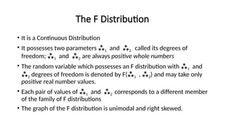
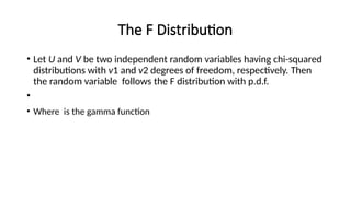
![The F Distribution
• E (F(1 , 2 )) = 2/(2-2) when 2 > 2
• V(F(1 , 2)) = 22
2
((1 + 2 - 2))/ (1)( 2 – 2)2
(2 - 4) when 2 > 4.
• It is undefined for 2 < 4.
• As 2 , the expression for the mean tends to 1 while the variance approaches
zero as both degrees of freedom become large.
• Define F( a : 1 , 2) & Define F( 1 - a: 2 , 1)
• Note that F( a : 1 , 2) = [F( 1 - a: 2 , 1)] –1
• Exercise 30: Use the Table of the F Distribution to compare the probabilities below
for (4,15) and (30,7) degrees of freedom
• P(F < 1.8) P( F > 2.4)](https://image.slidesharecdn.com/unit2probabilitydistributions1-240922165052-d94ea943/85/Unit-2-Probability-Distributions-1-pptx-86-320.jpg)


![[DSC Europe 25] Bojan Djuricic - Predictive Design Process.pdf](https://cdn.slidesharecdn.com/ss_thumbnails/5awdrbedqdek3gqu2ezy-4-the-predictive-design-bojan-djuricic-260120105856-6c399e9b-thumbnail.jpg?width=640&height=640&fit=bounds)


![[DSC Europe 25] Ivan Lukovic & Marija Djukic - From Data to Value: Why Maturi...](https://cdn.slidesharecdn.com/ss_thumbnails/ahrfps8xr6knowwhacxh-1-ivan-marija-dsc-2025-ld-v1-presentation-260115093812-be21adfc-thumbnail.jpg?width=640&height=640&fit=bounds)
