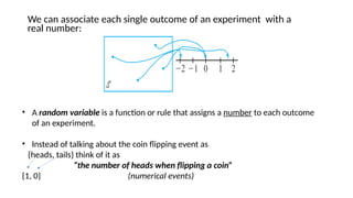
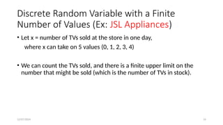
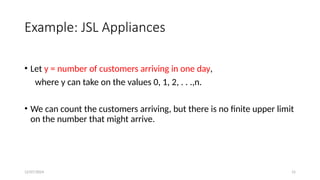
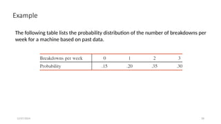
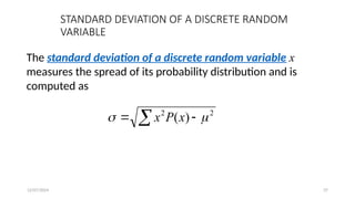
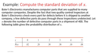
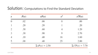
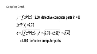
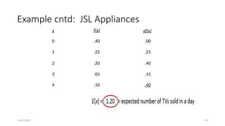
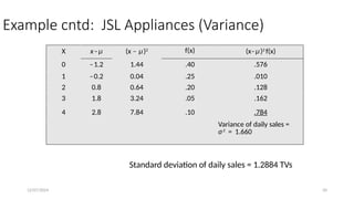
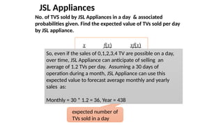
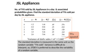
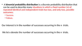
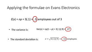
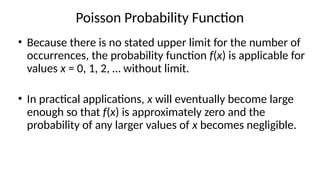
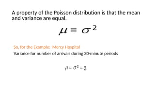
The document details the concepts of probability distributions and random variables, explaining their relevance in statistical analysis to summarize data and model uncertainties. It distinguishes between discrete and continuous random variables and provides examples of probability distributions related to real-world scenarios such as customer arrivals and product sales. Key statistical measures like expected value, variance, and standard deviation are also discussed with examples and their applications.

2. Business Statistics
PGDM (2023-24)
Term-II (Oct-Jan, 2023-24)
Ruchika Lochab
Assistant Professor, Operations
IMI, Delhi

3. 12/07/2024 3
Probability
Distributions

4. 12/07/2024
• Frequency distributions are a useful way of summarizing variations
in observed data. Frequency distributions by listing all the possible
outcomes of an experiment and then indicating the observed
frequency of each possible outcome.
• Probability distributions are related to frequency distributions. We
can think of a probability distribution as a theoretical
frequency distribution.
• A theoretical frequency distribution is a probability distribution
that describes how outcomes are expected to vary.

5. • Because these distributions deal with
expectations, they are useful models in making
inferences and decisions under conditions of
uncertainty.
• Probability distribution is related to random
experiments just like frequency distribution to
deterministic experiments.
• Frequency distribution is related to certainty in
outcome while probability distribution to

6. Examples
• Imagine you are rolling a fair six-sided die. The frequency distribution for
this experiment would show the counts of each possible outcome (1
through 6). The probability distribution would assign equal probabilities of
1/6 to each outcome, as each face of the die is equally likely.
• In the real world, you might collect data on the heights of individuals in a
population. The frequency distribution could show the number of people
within various height ranges. A probability distribution, such as the normal
distribution, could be used to model the probability of a randomly selected
person having a particular height.

7. 12/07/2024 7
In summary, probability distributions are essential tools for
understanding uncertainty and randomness in various fields.
They can be introduced and visualized using frequency
distributions, which provide a practical way to analyze and
interpret data collected from random experiments or
processes.

8. 12/07/2024 8
Unit 2: Probability Distributions
• 1 - Random Variables, Expected Value, Variance
• 2 - Discrete Probability Distributions
• 3 - Expected Value and Variance
• 4 - Binomial Probability Distribution
• 5 - Poisson Probability Distribution
• 6 - Continuous Probability Distributions
• 7 - Normal Probability Distributions
• 8 – Fat tail distributions
• 9 - Applications

9. Random Variables
Discrete Random Variables
Continuous Random Variables

10. 12/07/2024 10
Random Variables
• A random variable is a numerical description of the outcome of an
experiment.
• A discrete random variable may assume either a finite number of
values or an infinite sequence of values.
• A continuous random variable may assume any numerical value in an
interval or collection of intervals.

11. Probability Notations
An upper-case letter will represent the name of the random
variable, usually X.
Its lower-case counterpart will represent the value of the random
variable.
The probability that the random variable X will equal x is:
P(X = x) or more simply P(x)

12. We can associate each single outcome of an experiment with a
real number:
• A random variable is a function or rule that assigns a number to each outcome
of an experiment.
• Instead of talking about the coin flipping event as
{heads, tails} think of it as
“the number of heads when flipping a coin”
{1, 0} (numerical events)

13. 12/07/2024 13
Some Facts
• A random variable that may assume any numerical value in an interval
or collection of intervals is called a continuous random variable.
• Technically, relatively few random variables are truly continuous;
examples are values related to time, weight, distance, and
temperature.

14. 12/07/2024 14
Discrete Random Variable with a Finite
Number of Values (Ex: JSL Appliances)
• Let x = number of TVs sold at the store in one day,
where x can take on 5 values (0, 1, 2, 3, 4)
• We can count the TVs sold, and there is a finite upper limit on the
number that might be sold (which is the number of TVs in stock).

15. 12/07/2024 15
Example: JSL Appliances
• Let y = number of customers arriving in one day,
where y can take on the values 0, 1, 2, . . .,n.
• We can count the customers arriving, but there is no finite upper limit
on the number that might arrive.

16. 12/07/2024 16
Examples of Discrete Random Variables
Random Experiment Random Variable (x)
Possible Values for the Random
Variable
Flip a coin Face of a coin showing 1 if heads; 0 if tails
Roll a die Number of dots showing on top of
die
1, 2, 3, 4, 5, 6
Contact five customers Number of customers who place an
order
0, 1, 2, 3, 4, 5
Operate a health care clinic for one
day
Number of patients who arrive 0, 1, 2, 3, …
Offer a customer the choice of two
products
Product chosen by customer 0 if none; 1 if choose product A; 2 if
choose product B

17. 12/07/2024 17
Examples of Continuous Random Variables

18. 12/07/2024 18
Illustration Random Variable x Type
Family size x = Number of dependents reported on tax
return
Discrete
Distance from home to stores on a
highway
x = Distance in miles from home to the store
site
Continuous
Own dog or cat x = 1 if own no pet;
= 2 if own dog(s) only;
= 3 if own cat(s) only;
= 4 if own dog(s) and cat(s)
Discrete

19. 12/07/2024 19
A probability distribution (function) is a list of the probabilities of the values (simple
outcomes) of a random variable.
Table: Number of heads in two tosses of a coin
y p(y)
outcome probability
0 1/4
1 2/4
2 1/4
For some experiments, the probability of a simple outcome can
be easily calculated using a specific probability function. If y is a
simple outcome and p(y) is its probability.  


y
all
)
y
(
p
)
y
(
p
1
1
0
Probability Distribution

20. 12/07/2024 20
Example
 Each of the following tables lists certain values of x and their
probabilities. Determine whether or not each table represents a
valid probability distribution.

21. 12/07/2024 21
(a) No, since the sum of all probabilities is not equal to 1.0.
(b) Yes.
(c) No, since one of the probabilities is negative.
Solution

22. 12/07/2024 22
Discrete Probability
Distributions

23. Discrete Probability Distribution
The probability distribution for a random variable describes how
probabilities are distributed over the values of the random variable.
We can describe a discrete probability distribution with a table, graph,
or formula.
Types of discrete probability distributions:
First type: uses the rules of assigning probabilities to experimental
outcomes to determine probabilities for each value of the random
variable.
Second type: uses a special mathematical formula to compute the
probabilities for each value of the random variable.

24. 12/07/2024 24
Example
According to a survey, 60% of all students at a
university suffer from math anxiety. Two students are
randomly selected from this university. Let x denote
the number of students in this sample who suffer from
math anxiety. Develop the probability distribution of x.

25. 12/07/2024 25
Solution
Let us define the following two events:
 N = the student selected does not suffer from math
 anxiety
M = the student selected suffers from math anxiety
P(x = 0) = P(NN) = .16

P(x = 1) = P(NM or MN) = P(NM) + P(MN)
 = .24 + .24 = .48
 P(x = 2) = P(MM) = .36

26. 12/07/2024 26

27. 12/07/2024 27
Probability Distribution of the Number of Students with
Math Anxiety in a Sample of Two Students

28. 12/07/2024 28
Example
 The following table lists the probability distribution of the number of breakdowns per
week for a machine based on past data.

29. 12/07/2024 29
Example
(a) Present this probability distribution graphically.
(b) Find the probability that the number of breakdowns for this
machine during a given week is
i. exactly 2
ii. 0 to 2
iii. more than 1
iv. at most 1

30. 12/07/2024 30
Solution
• Let x denote the number of breakdowns for this machine during a
given week. Table below lists the probability distribution of x.

31. 12/07/2024 31
Solution: Graphical presentation of the
probability distribution of previous Table

32. 12/07/2024 32
Solution
(b) Using the Table,
i. P(exactly 2 breakdowns) = P(x = 2) = .35
ii. P(0 to 2 breakdowns) = P(0 ≤ x ≤ 2)
= P(x = 0) + P(x = 1) + P(x = 2)
= .15 + .20 + .35 = .70
iii. P(more then 1 breakdown) = P(x > 1)
= P(x = 2) + P(x = 3)
= .35 +.30 = .65
iv. P(at most one breakdown) = P(x ≤ 1)
= P(x = 0) + P(x = 1)
= .15 + .20 = .35

33. Mean (Expected Value)
• The mean is the weighted average of the values the random variable
may assume .The weights are the probabilities.
• This parameter is also called the expected value of X and is
represented by E(X).
• The expected value, or mean, of a random variable is a measure of its
central location.
• The expected value does not have to be a value the random variable
can assume.

34. Variance and Standard Deviation
The variance summarizes the variability in the
values of a random variable.
The variance is a weighted average of the squared
deviations of a random variable from its mean. The
weights are the probabilities. The standard deviation is
the square root of variance

35. 12/07/2024 35
Calculating mean for same example
In this table, x represents the number of breakdowns for a machine
during a given week, and P(x) is the probability of the corresponding
value of x.
Find the mean
number of
breakdowns per
week for this
machine.

36. 12/07/2024 36
Solution
The mean is µ = Σx P(x) = 1.80

37. 12/07/2024 37
STANDARD DEVIATION OF A DISCRETE RANDOM
VARIABLE
The standard deviation of a discrete random variable x
measures the spread of its probability distribution and is
computed as
 
 2
2
)
( 
 x
P
x

38. 12/07/2024 38
Example: Compute the standard deviation of x.
Baier’s Electronics manufactures computer parts that are supplied to many
computer companies. Despite the fact that two quality control inspectors at
Baier’s Electronics check every part for defects before it is shipped to another
company, a few defective parts do pass through these inspections undetected. Let
x denote the number of defective computer parts in a shipment of 400. The
following table gives the probability distribution of x.

39. 12/07/2024 39
Solution: Computations to Find the Standard Deviation

40. Solution Cntd.
 
 
2
2 2 2
2.50 defective computer parts in 400
( ) 7.70
7.70 (2.50) 1.45
1.204 defective computer parts
xP x
x P x
σ x P x


 
 
    




41. 12/07/2024 41
Example
 Loraine Corporation is planning to market a new makeup product. According to the
analysis made by the financial department of the company, it will earn an annual
profit of $4.5 million if this product has high sales and an annual profit of $ 1.2
million if the sales are mediocre, and it will lose $2.3 million a year if the sales are
low. The probabilities of these three scenarios are .32, .51 and .17 respectively.
(a) Let x be the profits (in millions of dollars) earned per annum from this
product by the company. Write the probability distribution of x.
(b) Calculate the mean and the standard deviation of x.

42. Solution
(a) The table below lists the probability distribution of x. Note that because x
denotes profits earned by the company, the loss is written as a negative
profit in the table.

43. Table: Computations to Find the Mean and Standard Deviation

44. Solution cntd.
(b) The Table shows all the calculations needed for the computation of the
mean and standard deviations of x.
 
 
million
314
.
2
$
)
661
.
1
(
1137
.
8
million
661
.
1
$
2
2
2











x
P
x
σ
x
P
x

45. The Statistical Abstract of the United States which publishes the report
annually… conducted a survey where US households are asked to report
the number of color televisions in the household. The following table
summarizes the data. Develop the probability distribution of the random
variable defined as the number of color televisions per household.
Number of Color Televisions Number of Households (1,000s)
0 1,218
1 32,379
2 37,961
3 19,387
4 7,714
5 2,842
Total 101,501
(1,218/101,501) = 0.012

46. 1. What is the probability that a randomly selected household has
no colour television?
P(X=0) = P(0) = 0.012=1.2%
2. What is the probability that a randomly selected household
owns two or more colour television?
P(X >=2) = P( X=2) +P(X=3)+ P(X=4) + P(X=5)
(From the addition rule of proability when the events are mutually exclusive)
3. what is the probability there is at least one television but no
more than three in any given household?
P(1 ≤ X ≤ 3) = P(1) + P(2) + P(3) = .319 + .374 + .191 = .884
X P(X)
0 0.012
1 0.319
2 0.374
3 0.191
4 0.076
5 0.028

47. 12/07/2024 47
Example: JSL Appliances
Using past data on TV sales, a tabular representation of the probability distribution
for sales was developed.
Units Sold
Number
of Days
0 80 0 .40 = 80/200
1 50 1 0.25
2 40 2 0.20
3 10 3 0.05
4 20 4 0.10
.
200
.
1.00

48. 12/07/2024 48
Example cntd: JSL Appliances

49. 12/07/2024 49
Example cntd: JSL Appliances
x f(x) xf(x)
0 .40 .00
1 .25 .25
2 .20 .40
3 .05 .15
4 .10 .40

50. 12/07/2024 50
Example cntd: JSL Appliances (Variance)
X x–μ (x – μ)2 f(x) (x–μ)2
f(x)
0 –1.2 1.44 .40 .576
1 –0.2 0.04 .25 .010
2 0.8 0.64 .20 .128
3 1.8 3.24 .05 .162
4 2.8 7.84 .10 .784
Variance of daily sales =
σ2
= 1.660
Standard deviation of daily sales = 1.2884 TVs

51. JSL Appliances
expected number of
TVs sold in a day
x f(x) xf(x)
0 .40 .00
1 .25 .25
2 .20 .40
3 .05 .15
4 .10 .40
E(x) = 1.20
No. of TVS sold by JSL Appliances in a day & associated
probabilities given. Find the expected value of TVs sold per day
by JSL appliance.
So, even if the sales of 0,1,2,3,4 TV are possible on a day,
over time, JSL Appliance can anticipate of selling an
average of 1.2 TVs per day. Assuming a 30 days of
operation during a month, JSL Appliance can use this
expected value to forecast average monthly and yearly
sales as:
Monthly = 30 * 1.2 = 36, Year = 438

52. JSL Appliances
No. of TVS sold by JSL Appliances in a day & associated
probabilities given. Find the standard deviation of TVs sold per
day by JSL appliance.
0
1
2
3
4
-1.2
-0.2
0.8
1.8
2.8
1.44
0.04
0.64
3.24
7.84
.40
.25
.20
.05
.10
.576
.010
.128
.162
.784
x -  (x - )2
f(x) (x - )2
f(x)
Variance of daily sales = s 2
= 1.660
x
TVs
squared
Standard deviation of daily sales = 1.2884 TVs
The standard deviation is measured in the same unit as the
random variable “TVs sold”. Variance is difficult to
interpret, so, STDEV is preferred to describe the variability
of a random variable.

53. Describing the Population of Monthly Profits
Monthly sales of computer store have a mean of $25,000 and a
standard deviation of $4,000. Profits are calculated by multiplying
sales by 30% and subtracting fixed costs of $6,000.
Find the mean monthly profit.
1) Describe the problem statement in algebraic terms:
sales have a mean of $25,000  E(Sales) = 25,000
profits are calculated by…
 Profit = .30(Sales) – 6,000

54. Laws of Expected Value
1. E(c) = c
The expected value of a constant (c) is just the value of
the constant.
2. E(X + c) = E(X) + c
3. E(cX) = cE(X)
We can “pull” a constant out of the expected value
expression (either as part of a sum with a random
variable X or as a coefficient of random variable X).

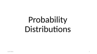
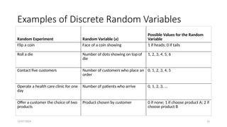
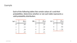
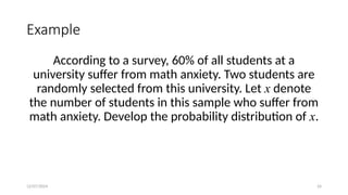
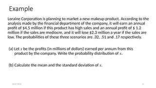
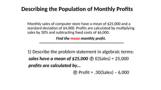
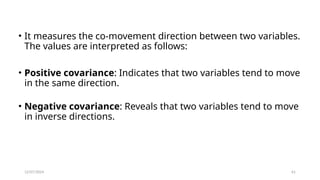
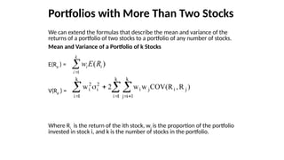
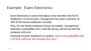
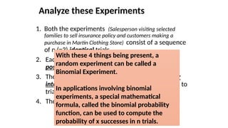
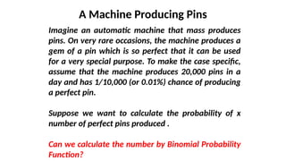
55. E(Profit) =E[.30(Sales) – 6,000]
=E[.30(Sales)] – 6,000
=.30E(Sales) – 6,000
=.30(25,000) – 6,000 = 1,500
Thus, the mean monthly profit is $1,500
Describing the Population of Monthly Profits
contd…

56. Monthly sales of a computer store have a mean of $25,000 and a
standard deviation of $4,000. Profits are calculated by multiplying
sales by 30% and subtracting fixed costs of $6,000.
Find the standard deviation of monthly profits.
1) sales have a standard deviation of $4,000
 V(Sales) = 4,0002
= 16,000,000 since
profits are calculated by…
 Profit = .30(Sales) – 6,000
Describing the Population of Monthly Profits

57. Laws of Variance
1. V(c) = 0
2. V(X + c) = V(X)
3. V(cX) = c2
V(X)

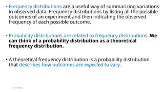
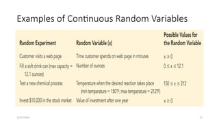
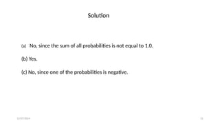
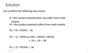
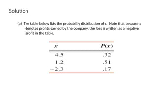
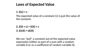
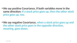
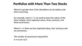
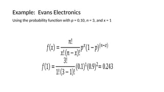
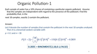
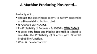
58. 2) The variance of profit is = V(Profit)
=V[.30(Sales) – 6,000]
=V[.30(Sales)]
=(.30)2
V(Sales)
=(.30)2
(16,000,000) = 1,440,000
so standard deviation of Profit
= (1,440,000)1/2
= $1,200
Describing the Population of Monthly Profits
contd…

59. 12/07/2024 59
APPLICATION IN FINANCIAL
MARKETS

60. 12/07/2024 60
Covariance
• Covariance is a measure of the relationship between two
random variables.
• The metric evaluates how much – to what extent – the
variables change together.
• In other words, it is essentially a measure of the variance
between two variables.
• However, the metric does not assess the dependency
between variables.

61. 12/07/2024 61
• It measures the co-movement direction between two variables.
The values are interpreted as follows:
• Positive covariance: Indicates that two variables tend to move
in the same direction.
• Negative covariance: Reveals that two variables tend to move
in inverse directions.

62. 12/07/2024 62
• We say positive Covariance, if both variables move in the
same direction: If a stock price goes up, then the other stock
price goes up, too.
• We say negative Covariance, when a stock price goes up and
the other stock price goes in the opposite direction,
meaning, goes down.

63. 12/07/2024 63
• In finance, the concept is primarily used in portfolio theory.
• One of its most common applications in portfolio theory is
the diversification method, using the covariance between
assets in a portfolio.
• By choosing assets that do not exhibit a high positive
covariance with each other, the unsystematic risk can be
partially eliminated.

64. 12/07/2024 64
Formula
The covariance between two random variables X and Y can be calculated using the above
formula.
Where:
•Xi – the values of the X-variable
•Yj – the values of the Y-variable
•X
̄ – the mean (average) of the X-variable
•Ȳ – the mean (average) of the Y-variable
•n – the number of data points

65. Portfolios with More Than Two Stocks
We can extend the formulas that describe the mean and variance of the
returns of a portfolio of two stocks to a portfolio of any number of stocks.
Mean and Variance of a Portfolio of k Stocks
E(Rp ) =
V(Rp ) =
Where Ri is the return of the ith stock, wi is the proportion of the portfolio
invested in stock i, and k is the number of stocks in the portfolio.


k
i
i
i R
E
w
1
)
(
 
  




k
1
i
k
1
i
j
j
i
j
i
k
1
i
2
i
2
i )
R
,
R
(
COV
w
w
2
w

66. Portfolios with More Than Two Stocks
When k is greater than 2 the calculations can be tedious and
time-consuming.
For example, when k = 3, we need to know the values of the
three weights, three expected values, three variances, and
three covariances.
When k = 4, there are four expected values, four variances and
six covariances.
The number of covariances required for
k =n is n(n-1)/2

67. Investment Decision
An investor has $100,000 to invest in the stock market. She is
interested in developing a stock portfolio made up of General Electric,
General Motors, McDonald’s, and Motorola. However, she doesn’t
know how much to invest in each one. She wants to maximize her
return, but she would also like to minimize the risk. She has computed
the monthly returns for all four stocks during a 60-month period
(January 2017 to December 2022)
After some consideration, she narrowed her choices down to the following
three. What should she do?
1. $25,000 in each stock (equal weightage)
2. General Electric: $10,000, General Motors: $20,000, McDonald’s: $30,000,
Motorola: $40,000
3. General Electric: $10,000, General Motors: $50,000, McDonald’s: $30,000,
Motorola: $10,000
Microsoft Office
Excel Worksheet
Microsoft Office
Word Document

68. Discrete Probability
Distributions:
Binomial Distribution

69. • A binomial probability distribution is a discrete probability distribution that
can be used to describe many situations in which a fixed number (n) of
repeated identical and independent trials has two, and only two, possible
outcomes:
• Success.
• Failure.
Our interest is in the number of successes occurring in the n trials.
We let x denote the number of successes occurring in the n trials.

70. Four Properties of a Binomial
Experiment
1. The experiment consists of a sequence of n identical trials.
2. Two outcomes, success and failure, are possible on each trial.
3. The probability of a success, denoted by p, does not change from
trial to trial.
4. The trials are independent.
Prop 3 is called
stationarity
assumption
If Property 2, 3 and 4 are present, then the underlying process is
called Bernoulli Process. If in addition, property 1 is present,
then it becomes a binomial experiment

71. Binomial Probability Distribution
Binomial Probability Function
where:
x = the number of successes
p = the probability of a success on one trial
n = the number of trials
f(x) = the probability of x successes in n trials

72. Binomial Probability Distribution
Binomial Probability Function

73. 12/07/2024 73
Example: Evans Electronics
Evans Electronics is concerned about a low retention rate for its
employees. In recent years, management has seen a turnover of
10% of the hourly employees annually.
Thus, for any hourly employee chosen at random, management
estimates a probability of 0.1 that the person will not be with the
company next year.
Choosing 3 hourly employees at random, what is the probability that
1 of them will leave the company this year?

74. Example: Evans Electronics
Using the probability function with p = 0.10, n = 3, and x = 1

75. Example: Evans Electronics (Tree Diagram)

76. Formulae
• The expected value is:
• The variance is:
• The standard deviation is:

77. Applying the formulae on Evans Electronics
• The variance is:
• The standard deviation is:

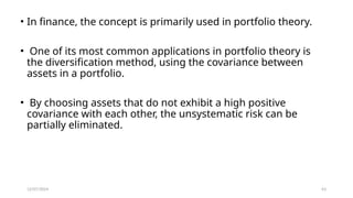
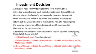
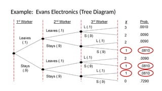
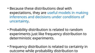
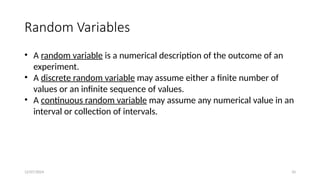
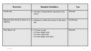
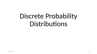
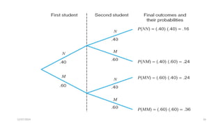
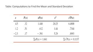
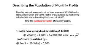
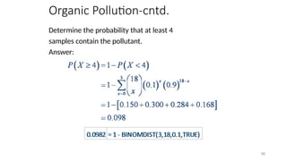
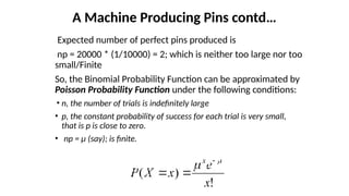
78. Evans Electronics Using EXCEL
Type the following into an empty cell.
= BINOMIDIST([x], [n], [p], [TRUE], [FALSE])
Typing ‘true’ calculates cumulative probability
distribution (say F(5)= P(x<=5)=Pr at most 5 occurrences
or successes).
Typing ‘false’ computes the probability of an individual
value of x , for example P(x=5)

79. Evans Electronics Using EXCEL

80. Selling Insurance Policy
Consider an insurance salesperson who visits 3 randomly selected families in a
locality. The outcome associated with each visit is either family purchases the
insurance policy or does not purchase. Past experience suggests that there is 10%
chance that a randomly selected family will purchase an insurance policy.
What is the probability that 2 families will make a purchase?
(Looks like this one can be solved by drawing a tree diagram)
Suppose now the salesperson visits 10, 50 and then 100 families. How can we find
the probability that 5 or more families will purchase insurance policy?
(Can we solve this just drawing a tree diagram or need some rule/formula?)

81. Insurance Policy: Tree Diagram
1st
Family 2nd
Family 3rd
Family x Outcome
Purchases (S)
(.1)
Does not (F)
(.9)
3
2
0
2
2
Purchases (.1) (S)
Purchases (S) (.1)
(.9) (F)
Does not (.9) (F)
Does not (.9) (F)
(.9) (F)
(.9) (F)
(.9) (F)
(.1) (S)
(.1) (S)
(.1) (S)
(.1) (S) (S,S,S)
(S,F,S)
(F,S,S)
(F,F,F)
(S,S,F)
1
1
(S,F,F)
(F,S,F)
(F,F,S)
1
To find the prob that 2 families will
purchase the policies...
- Find the possible outcomes
-Find the joint probabilities
- and then add

82. Insurance Policy: Tree Diagram
1st
Family 2nd
Family 3rd
Family x
Purchases (S)
(.1)
Does not (F)
(.9)
3
2
0
2
2
Purchases (.1) (S)
Purchases (S) (.1)
(.9) (F)
Does not (.9) (F)
Does not (.9) (F)
(.9) (F)
(.9) (F)
(.9) (F)
(.1) (S)
(.1) (S)
(.1) (S)
(.1) (S)
1
1
1
To find the prob that 2 families will
purchase the policies…
3*0.0090 = 0.027
Prob.
.0010
.0090
.0090
.7290
.0090
.0810
.0810
.0810
How can you find the prob that 5 or more families will make a
purchase when the salesperson visits 50 families

83. Martin Clothing Store Problem
Consider the purchase decisions of the next three customers who enter the
Martin Clothing Store. On the basis of past experience, the store manager
estimates that the probability that any one customer will make a purchase
is 0.30.
What is the probability that one of next three customers will make a
purchase? (again, a tree diagram can help to get the answer!)
Suppose now Martin Store wants to find out of next 100 customers, what
would be the probability that 3 or more customers will make a purchase?
(Does not look like a tree diagram can be of much help here!!!)

84. Martin Clothing Store: Tree Diagram
1st
Customer 2nd
Customer 3rd
Customer x Outcome
Purchases (S)
(.30)
Not (F)
(.70)
3
2
0
2
2
S (.30)
F (.70)
(S,S,S)
(S,F,S)
(F,S,S)
(F,F,F)
(S,S,F)
1
1
(S,F,F)
(F,S,F)
(F,F,S)
1
S (.30)
F (.70)
S (.30)
F (.70)
S (.30)
F (.70)
S (.30)
F (.70)
S (.30)
F (.70)

85. Martin Clothing Store: Tree Diagram
1st
Customer 2nd
Customer 3rd
Customer x
Purchases (S)
(.30)
Not (F)
(.70)
3
2
0
2
2
S (.30)
F (.70)
1
1
1
S (.30)
F (.70)
S (.30)
F (.70)
S (.30)
F (.70)
S (.30)
F (.70)
S (.30)
F (.70)
Prob.
.027
.063
.063
.343
.063
.147
.147
.147
To find the prob that 1 customer will
purchase
3*0.147= 0.441
How can you find the prob that 3 or more customers will make a
purchase in the next 100 customers

86. Analyze these Experiments
1. Both the experiments (Salesperson visiting selected
families to sell insurance policy and customers making a
purchase in Martin Clothing Store) consist of a sequence
of n (=3) identical trials.
2. Each trial of these two experiments has two
possible outcomes.
3. The probability of a success (or the event of our
interest), denoted by p, remains same from trial to
trial 0.1 for exp 1 and 0.3 for exp 2.
4. The trials are independent.
With these 4 things being present, a
random experiment can be called a
Binomial Experiment.
In applications involving binomial
experiments, a special mathematical
formula, called the binomial probability
function, can be used to compute the
probability of x successes in n trials.

87. Organic Pollution-1
Each sample of water has a 10% chance of containing a particular organic pollutant. Assume
that the samples are independent with regard to the presence of the pollutant. Find the
probability that, in the
next 18 samples, exactly 2 contain the pollutant.
Answer:
Let X denote the number of samples that contain the pollutant in the next 18 samples analyzed.
Then X is a binomial random variable with
p = 0.1 and n = 18
87

88. Organic Pollution-cntd.
Determine the probability that at least 4
samples contain the pollutant.
Answer:
88

89. Organic Pollution-cntd.
Now determine the probability that 3 ≤ X < 7.
Answer:
89
Appendix A, Table II (pg. 705) is a cumulative binomial table for
selected values of p and n.

90. Discrete Probability
Distributions:
Poisson Distribution

91. 12/07/2024 91
Poisson Probability Distribution
• A discrete random variable that is often useful in estimating the number of
occurrences of an event over a specified interval of time and space.
• Examples:
• Number of patients who arrive at a health care clinic in one hour.
• Number of computer-server failures in a month.
• Number of repairs needed in 10 miles of highway.
• Number of leaks in 100 miles of pipeline.
• number of vehicles arriving at a toll booth in one hour

92. Poisson Probability Distribution
• It is a discrete random variable that may assume an infinite
sequence of values (x = 0, 1, 2, . . . ).
• Bell Labs used the Poisson distribution to model the arrival of
phone calls.

93. Two Properties of a Poisson Experiment
1. The probability of an occurrence is the same for any two intervals of equal length.
2. The occurrence or nonoccurrence in any interval is independent of the occurrence or
nonoccurrence in any other interval.
Poisson Probability Function:
where:
x = the number of occurrences in an interval
f(x) = the probability of x occurrences in an interval
μ = mean number of occurrences in an interval
e ≈ 2.71828
x! = x(x – 1)(x – 2) . . . (2)(1)

94. Poisson Probability Function
• Because there is no stated upper limit for the number of
occurrences, the probability function f(x) is applicable for
values x = 0, 1, 2, … without limit.
• In practical applications, x will eventually become large
enough so that f(x) is approximately zero and the
probability of any larger values of x becomes negligible.

95. Mean and Variance of Poisson
Distribution
A property of the Poisson distribution is that the mean and variance are equal.
np = np(1-p);
The RHS of above expression is Binomial Variance. In case of Poisson
distribution, p is very small, so, 1-p is close to 1. So, variance of a Poisson
distribution becomes np, same as mean.
μ = σ2
In this case, we will write, if X ~ P(μ);
where μ is the expected value of the distribution.
So, for Poisson Distribution, all one needs to know is the expected value of the
distribution.

96. 12/07/2024 96
Example: Mercy Hospital
Patients arrive at the emergency room of Mercy Hospital at the average rate of 6 per
hour on weekend evenings.
What is the probability of 4 arrivals in 30 minutes on a weekend evening?
Using the probability function with = 6/hour = 3/half-hour and x = 4

98. A property of the Poisson distribution is that the mean
and variance are equal.
So, for the Example: Mercy Hospital
Variance for number of arrivals during 30-minute periods

99. Mercy Hospital Using Excel

100. Calculations for Wire Flaws
For the case of the thin copper wire, suppose that the number of flaws follows
a Poisson distribution. With a mean of 2.3 flaws per mm. Find the
probability of exactly 2 flaws in 1 mm of wire.
Answer:
Let X denote the number of flaws in 1 mm of wire
100

101. Calculations for Wire Flaws-cntd.
Determine the probability of 10 flaws in 5 mm of
wire.
Answer :
Let X denote the number of flaws in 5 mm of wire.
Sec 3-9 Poisson Distribution 101

102. A Machine Producing Pins
Imagine an automatic machine that mass produces
pins. On very rare occasions, the machine produces a
gem of a pin which is so perfect that it can be used
for a very special purpose. To make the case specific,
assume that the machine produces 20,000 pins in a
day and has 1/10,000 (or 0.01%) chance of producing
a perfect pin.
Suppose we want to calculate the probability of x
number of perfect pins produced .
Can we calculate the number by Binomial Probability
Function?

103. Probably not….
• Though the experiment seems to satisfy properties
of a Binomial distribution….but
• N =20000 ; VERY LARGE
• P = Probability of Success = 1/10000 is VERY SMALL
• N being very large and P being so small, it is hard to
calculate the Probability of Success with Binomial
Probability Function.
• What is the alternative?
A Machine Producing Pins contd…

104. Expected number of perfect pins produced is
np = 20000 * (1/10000) = 2; which is neither too large nor too
small/Finite
So, the Binomial Probability Function can be approximated by
Poisson Probability Function under the following conditions:
• n, the number of trials is indefinitely large
• p, the constant probability of success for each trial is very small,
that is p is close to zero.
• np = µ (say); is finite.
A Machine Producing Pins contd…
!
)
(
x
e
x
X
P
x 
 


!
)
(
x
e
x
X
P
x 
 



105. Thanks!

106. Extra Slides

107. Binomial Probability Distribution
Using Tables of Binomial Probabilities
n x p = .05 p = .10 p = .15 p = .20 p = .25 p =.30 p = .35 p =.40 p =.45 p =.50
3 0 .8574 .7290 .6141 .5120 .4219 .3430 .2746 .2160 .1664 .1250
3 1 .1354 .2430 .3251 .3840 .4219 .4410 .4436 .4320 .4084 .3750
3 2 .0071 .0270 .0574 .0960 .1406 .1890 .2389 .2880 .3341 .3750
3 3 .0001 .0010 .0034 .0080 .0156 .0270 .0429 .0640 .0911 .1250