Slides for the class on Probability Distributions

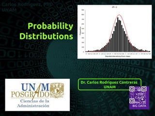
1. Dr. Carlos Rodríguez Contreras
UNAM
Probability
Distributions

2. Probability Distributions
 A probability distribution is a mathematical function
that provides the probabilities of occurrence of
different possible outcomes in an experiment.
 In more technical terms, the probability distribution
is a description of a random phenomenon in terms of
the probabilities of events.
 For instance, if the random variable X is used to
denote the outcome of a coin toss ("the
experiment"), then the probability distribution of X
would take the value 0.5 for X = heads, and 0.5 for X =
tails.

3. Probability Distributions
 Random Variable
 Represents a possible numerical value from a random event
 Takes on different values based on chance
Random
Variables
Discrete
Random Variable
Continuous
Random Variable

4. Probability Distributions Gallery

5.  A discrete random variable is a variable that can
assume only a countable number of values
 Many possible outcomes:
 number of complaints per day
 number of TV’s in a household
 number of rings before the phone is answered
 Only two possible outcomes:
 gender: male or female
 defective: yes or no
Discrete Random Variables

6. Discrete Random Variables
 Can only assume a countable number of values
Examples:
– Roll a die twice
Let x be the number of times 4 comes up
(then x could be 0, 1, or 2 times)
– Toss a coin 5 times.
Let x be the number of heads
(then x = 0, 1, 2, 3, 4, or 5)

7. x Value Probability
0 1/4 = .25
1 2/4 = .50
2 1/4 = .25
Experiment: Toss 2 Coins. Let x = # heads.
T
T
Discrete Probability Distributions
4 possible outcomes
T
T
Probability Distribution
0 1 2 x
.50
.25
Probability

8. Discrete Probability Distributions
A videoclip by Ben Lambert

9. Examples of some of the most known
Discrete Probability Distributions

10. Bernoulli Distribution
 The Bernoulli distribution is a binomial distribution with n=1, and one instance
of a Bernoulli distribution is called a Bernoulli trial.
 One coin flip is a Bernoulli trial, for example.

11. Binomial Distribution
 The binomial distribution is a discrete probability distribution. It describes the
outcome of n independent trials in an experiment. Each trial is assumed to have
only two outcomes, either success or failure. If the probability of a successful
trial is p, then the probability of having x successful outcomes in an experiment
of n independent trials is as follows.

12. Binomial Distribution
 Suppose there are twelve multiple choice questions in an English class quiz. Each
question has five possible answers, and only one of them is correct. Find the
probability of having four or less correct answers if a student attempts to answer
every question at random.
 Solution
Since only one out of five possible answers is correct, the probability of
answering a question correctly by random is 1/5=0.2. We can find the probability
of having exactly 4 correct answers by random attempts as follows.
> dbinom(4, size=12, prob=0.2)
[1] 0.1329

13. Binomial Distribution
 To graph all possible results, we need a vector with all possibilities:

14. Geometric Distribution
 Geometric distributions model (some) discrete random variables. Typically, a
Geometric random variable is the number of trials required to obtain the first
failure, for example, the number of tosses of a coin until the first 'tail' is
obtained, or a process where components from a production line are tested, in
turn, until the first defective item is found.
 A discrete random variable X is said to follow a Geometric distribution with
parameter p, written X ~ Ge(p):
P(X=x) = px-1(1-p)x
where
x = 1, 2, 3, ...
p = success probability; 0 < p < 1

15. Geometric Distribution
 The trials must meet the following requirements:
 the total number of trials is potentially infinite;
 there are just two outcomes of each trial; success and failure;
 the outcomes of all the trials are statistically independent;
 all the trials have the same probability of success.
 The Geometric distribution is related to the Binomial distribution in that both
are based on independent trials in which the probability of success is constant
and equal to p. However, a Geometric random variable is the number of trials
until the first failure, whereas a Binomial random variable is the number of
successes in n trials.

16. Poisson Distribution
 The Poisson distribution is the probability distribution of independent event
occurrences in an interval. If λ is the mean occurrence per interval, then the
probability of having x occurrences within a given interval is:

17. Poisson Distribution
 If there are twelve cars crossing a bridge per minute on average, find the probability of
having seventeen or more cars crossing the bridge in a particular minute.
 Solution
The probability of having sixteen or less cars crossing the bridge in a particular minute is
given by the function ppois.
> ppois(16, lambda=12) # lower tail
[1] 0.89871
 Hence the probability of having seventeen or more cars crossing the bridge in a minute is
in the upper tail of the probability density function.
> ppois(16, lambda=12, lower=FALSE) # upper tail
[1] 0.10129

18. Poisson Distribution
 To graph all possible results, we need a vector with all possibilities:

19. Exponential Distribution
 The exponential distribution describes the arrival time of a randomly recurring
independent event sequence. If μ is the mean waiting time for the next event
recurrence, its probability density function is:

20. Exponential Distribution
 Suppose the mean checkout time of a supermarket cashier is three minutes. Find
the probability of a customer checkout being completed by the cashier in less
than two minutes.
 Solution
The checkout processing rate is equals to one divided by the mean checkout
completion time. Hence the processing rate is 1/3 checkouts per minute. We then
apply the function pexp of the exponential distribution with rate=1/3.
> pexp(2, rate=1/3)
[1] 0.48658

21. Exponential Distribution
 To graph density of probabilities, we need a vector with all possibilities:

22. Exponential Distribution
 To graph all possible results, we need a vector with all possibilities:

23. Continuous Probability Distributions

24. Continuous Random Variables
 A continuous random variable is a variable that can
assume any value on a continuum (can assume an
uncountable number of values)
 thickness of an item
 time required to complete a task
 temperature of a solution
 height, in inches
 These can potentially take on any value, depending
only on the ability to measure accurately.

25. Represented by a PDF (Probability Density
Function)
P(x) = Probability in a range of values
x’s are mutually exclusive
(no overlap)
x’s are collectively exhaustive
(nothing left out)
0 < P(x) < 1 for each range of x
S P(x) = 1
Continuous Probability Distributions

26. A videoclip by JBstatistics

27. The Normal Distribution

28. Normal Distribution PDF
 The normal distribution is defined by the following probability density function,
where μ is the population mean and σ2 is the variance.

29. Normal Distribution and CLT
 The normal distribution is important because of the Central Limit Theorem,
which states that the population of all possible samples of size n from a
population with mean μ and variance σ2 approaches a normal distribution with
mean μ and σ2∕n when n approaches infinity.

30. A videoclip by Ben Lambert...

31. Normal Distribution Props
‘Bell Shaped’
Symmetrical
Mean, Median and Mode are Equal
Location is determined by the mean, μ
Spread is determined by the standard
deviation, σ
The random variable has an infinite
theoretical range:
+ to - 
Mean
= Median
= Mode
x
f(x)
μ
σ

32. By varying the parameters μ and σ, we obtain different normal distributions
Many Normal Distributions

33. The Normal Distribution Shape
x
f(x)
μ
σ
Changing μ shifts the
distribution left or right.
Changing σ increases
or decreases the
spread.

34. A videoclip of Joshua Starmer from
StatQuest!!!

35. Finding Normal Probabilities
a b x
f(x)
P a x b( ) 
Probability is measured by the area
under the curve

36. Probability as the
Area Under the Curve
The total area under the curve is 1.0, and the curve is
symmetric, so half is above the mean, half is below
1.0)xP(  
f(x)
xμ
0.50.5
0.5μ)xP( =<<- ¥
0.5)xP(μ =¥<<

37.  If the data distribution is bell-shaped, then the
interval:
 contains about 68% of the values in the sample
The Empirical Rule
1σμ 

38.  If the data distribution is bell-shaped, then the
interval:
 contains about 95% of the values in the sample
The Empirical Rule
2σμ 

39.  If the data distribution is bell-shaped, then the
interval:
 contains about 99.7% of the values in the sample
The Empirical Rule
3σμ 

40. Importance of the Rule
 If a value is about 2 or more standard deviations
away from the mean in a normal distribution, then it
is far from the mean.
 The chance that a value that far or farther away from
the mean is highly unlikely, given that particular
mean and standard deviation.

41. Probability Distributions
A reinforcement

42. Let us try all these in
Work with empiricalRule.R

43. Normal Distribution Exercise
 Assume that the test scores of a college entrance exam fits a normal distribution.
Furthermore, the mean test score is 72, and the standard deviation is 15.2. What
is the percentage of students scoring 84 or more in the exam?
 Solution
We apply the function pnorm of the normal distribution with mean 72 and
standard deviation 15.2. Since we are looking for the percentage of students
scoring higher than 84, we are interested in the upper tail of the normal
distribution.
> pnorm(84, mean=72, sd=15.2, lower.tail=FALSE)
[1] 0.21492

44. Normal Distribution

45. Normal and proofs of normality
Work with NormalDist.R