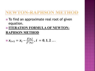
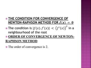
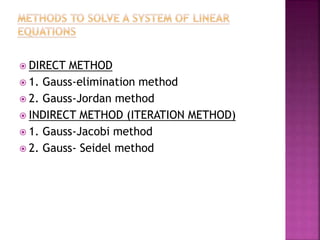
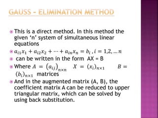
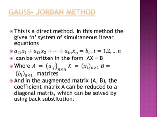
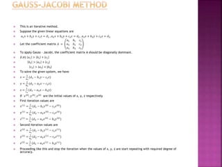
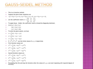
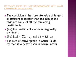
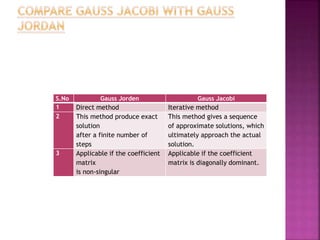
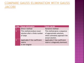
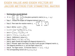
 To find an approximate real root of given
equation.
 ITERATION FORMULA OF NEWTON-
RAPHSON METHOD
 𝒙𝒊+𝟏 = 𝒙𝒊 −
𝒇 𝒙 𝒊
𝒇′ 𝒙 𝒊
, 𝒊 = 𝟎, 𝟏, 𝟐 … .
 THE CONDITION FOR CONVERGENCE OF
NEWTON-RAPHSON METHOD FOR 𝒇(𝒙) = 𝟎
 The condition is |𝑓(𝑥). 𝑓′(𝑥)| < 𝑓′ 𝑥
2
in a
neighbourhood of the root
 ORDER OF CONVERGENCE OF NEWTON-
RAPHSON METHOD
 The order of convergence is 2.
 To find the root of the equation 𝑓(𝑥) = 0
 Step 1. Find the numbers a and b in such a way that
𝑓(𝑎) and 𝑓(𝑏) are in opposite signs. (From this we
conclude that there is one real root between a and b)
 Step 2. Choose the initial approximate root as 𝑥0
 Step 3. Using the Newton Raphson’s formula 𝒙𝒊+𝟏 =
𝒙𝒊 −
𝒇 𝒙𝒊
𝒇′ 𝒙 𝒊
, 𝒊 = 𝟎, 𝟏, 𝟐 … ., find the sequence
𝑥0, 𝑥1, … 𝑥 𝑛, . . and the point of convergence of the
sequence is the root of the given equation.
 1. It can be used for finding root of both
algebraic and transcendental equations.
 2. The convergence of Newton’s method is
faster and so it is preferred compared to
other methods.
 3. It is simple and easy to deal with and it is
used to improve the results obtained by
other methods.
 To find the root of the equation 𝑓(𝑥) = 0
 Step 1. Find the numbers a and b in such a way that
𝑓(𝑎) and 𝑓(𝑏) are in opposite signs. (From this we
conclude that there is one real root between a and b)
 Step 2. Write the given equation on the form 𝑥 =
∅(𝑥)
 Step 3. Choose the initial approximate root as 𝑥0
 Step 4. Replace 𝑥 by 𝑥0 in step 2, and take 𝑥1 =
∅(𝑥0)
 Step 5. Further , find 𝑥2 = ∅(𝑥1)
 Step 6. Continuing this way, we will get a sequence
𝑥0, 𝑥1, … 𝑥 𝑛, . . and the point of convergence of the
sequence is the root of the given equation
 ORDER OF CONVERGENCE OF FIXED POINT
ITERATION METHOD
 The order of convergence is 1.
 THE CONDITION FOR CONVERGENCE OF
FIXED POINT ITERATION METHOD FOR
𝒇(𝒙) = 𝟎
 The condition is |∅′ 𝑥 | < 1, for all values of
𝑥
 DIRECT METHOD
 1. Gauss-elimination method
 2. Gauss-Jordan method
 INDIRECT METHOD (ITERATION METHOD)
 1. Gauss-Jacobi method
 2. Gauss- Seidel method
 This is a direct method. In this method the
given ‘n’ system of simultaneous linear
equations
 𝑎𝑖1 𝑥1 + 𝑎𝑖2 𝑥2 + ⋯ + 𝑎𝑖𝑛 𝑥 𝑛 = 𝑏𝑖 , 𝑖 = 1,2, … 𝑛
 can be written in the form AX = B
 Where 𝐴 = 𝑎𝑖𝑗 𝑛×𝑛
𝑋 = 𝑥𝑖 𝑛×1 𝐵 =
𝑏𝑖 𝑛×1 matrices
 And in the augmented matrix (A, B), the
coefficient matrix A can be reduced to upper
triangular matrix, which can be solved by
using back substitution.
 This is a direct method. In this method the
given ‘n’ system of simultaneous linear
equations
 𝑎𝑖1 𝑥1 + 𝑎𝑖2 𝑥2 + ⋯ + 𝑎𝑖𝑛 𝑥 𝑛 = 𝑏𝑖 , 𝑖 = 1,2, … 𝑛
 can be written in the form AX = B
 Where 𝐴 = 𝑎𝑖𝑗 𝑛×𝑛
𝑋 = 𝑥𝑖 𝑛×1 𝐵 =
𝑏𝑖 𝑛×1 matrices
 And in the augmented matrix (A, B), the
coefficient matrix A can be reduced to a
diagonal matrix, which can be solved by
using back substitution.
 This is an iterative method.
 Suppose the given linear equations are
 𝑎1 𝑥 + 𝑏1 𝑦 + 𝑐1 𝑧 = 𝑑1 , 𝑎2 𝑥 + 𝑏2 𝑦 + 𝑐2 𝑧 = 𝑑2 , 𝑎3 𝑥 + 𝑏3 𝑦 + 𝑐3 𝑧 = 𝑑3
 Let the coefficient matrix 𝐴 =
𝑎1 𝑏1 𝑐1
𝑎2 𝑏2 𝑐2
𝑎3 𝑏3 𝑐3
 To apply Gauss – Jacobi, the coefficient matrix A should be diagonally dominant.
 (i.e) 𝑎1 > 𝑏1 + 𝑐1
 𝑏2 > 𝑎2 + 𝑐2
 𝑐3 > 𝑎3 + |𝑏3|
 To solve the given system, we have
 𝑥 =
1
𝑎1
(𝑑1 − 𝑏1 𝑦 − 𝑐1 𝑧)
 𝑦 =
1
𝑏2
(𝑑2 − 𝑎2 𝑥 − 𝑐2 𝑧)
 𝑧 =
1
𝑐3
(𝑑3 − 𝑎3 𝑥 − 𝑏3 𝑦)
 If 𝑥(0), 𝑦(0), 𝑧(0) are the initial values of x, y, z respectively
 First iteration values are
 𝑥 1 =
1
𝑎1
(𝑑1 − 𝑏1 𝑦 0 − 𝑐1 𝑧 0 )
 𝑦 1 =
1
𝑏2
(𝑑2 − 𝑎2 𝑥 0 − 𝑐2 𝑧 0 )
 𝑧 1 =
1
𝑐3
(𝑑3 − 𝑎3 𝑥 0 − 𝑏3 𝑦 0 )
 Second iteration values are
 𝑥 2 =
1
𝑎1
(𝑑1 − 𝑏1 𝑦 1 − 𝑐1 𝑧 1 )
 𝑦 2 =
1
𝑏2
(𝑑2 − 𝑎2 𝑥 1 − 𝑐2 𝑧 1 )
 𝑧 2 =
1
𝑐3
(𝑑3 − 𝑎3 𝑥 1 − 𝑏3 𝑦 1 )
 Proceeding like this and stop the iteration when the values of x, y, z are start repeating with required degree of
accuracy.
 This is an iterative method.
 Suppose the given linear equations are
 𝑎1 𝑥 + 𝑏1 𝑦 + 𝑐1 𝑧 = 𝑑1 , 𝑎2 𝑥 + 𝑏2 𝑦 + 𝑐2 𝑧 = 𝑑2 , 𝑎3 𝑥 + 𝑏3 𝑦 + 𝑐3 𝑧 = 𝑑3
 Let the coefficient matrix 𝐴 =
𝑎1 𝑏1 𝑐1
𝑎2 𝑏2 𝑐2
𝑎3 𝑏3 𝑐3
 To apply Gauss – Seidel, the coefficient matrix A should be diagonally dominant.
 (i.e) 𝑎1 > 𝑏1 + 𝑐1
 𝑏2 > 𝑎2 + 𝑐2
 𝑐3 > 𝑎3 + |𝑏3|
 To solve the given system, we have
 𝑥 =
1
𝑎1
(𝑑1 − 𝑏1 𝑦 − 𝑐1 𝑧)
 𝑦 =
1
𝑏2
(𝑑2 − 𝑎2 𝑥 − 𝑐2 𝑧)
 𝑧 =
1
𝑐3
(𝑑3 − 𝑎3 𝑥 − 𝑏3 𝑦)
 If 𝑥(0), 𝑦(0), 𝑧(0) are the initial values of x, y, z respectively
 First iteration values are
 𝑥 1 =
1
𝑎1
(𝑑1 − 𝑏1 𝑦 0 − 𝑐1 𝑧 0 )
 𝑦 1 =
1
𝑏2
(𝑑2 − 𝑎2 𝑥 1 − 𝑐2 𝑧 0 )
 𝑧 1 =
1
𝑐3
(𝑑3 − 𝑎3 𝑥 1 − 𝑏3 𝑦 1 )
 Second iteration values are
 𝑥 2 =
1
𝑎1
(𝑑1 − 𝑏1 𝑦 1 − 𝑐1 𝑧 1 )
 𝑦 2 =
1
𝑏2
𝑑2 − 𝑎2 𝑥 2 − 𝑐2 𝑧 1
 𝑧 2 =
1
𝑐3
(𝑑3 − 𝑎3 𝑥 2 − 𝑏3 𝑦 2 )
 Proceeding like this and stop the iteration when the values of x, y, z are start repeating with required degree of
accuracy.
 The condition is the absolute value of largest
coefficient is greater than the sum of the
absolute value of all the remaining
coefficients.
 (i.e) the coefficient matrix is diagonally
dominant
 (i.e) 𝑎𝑖𝑖 > 𝑗=1,𝑖≠𝑗
𝑛
|𝑎𝑖𝑗| ∀ 𝑖 = 1,2 … 𝑛
 The rate of convergence in Gauss –Seidel
method is very fast than in Gauss-Jacobi
S.No Gauss Jorden Gauss Jacobi
1 Direct method Iterative method
2 This method produce exact
solution
after a finite number of
steps
This method gives a sequence
of approximate solutions, which
ultimately approach the actual
solution.
3 Applicable if the coefficient
matrix
is non-singular
Applicable if the coefficient
matrix is diagonally dominant.
S.No Gauss elimination Gauss Jacobi
1 Direct method Iterative method
2 This method produce exact
solution after a finite number
of steps
This method gives a sequence
of approximate solutions,
which ultimately approach the
actual solution.
3 Applicable if the coefficient
matrix
is non-singular
Applicable if the coefficient
matrix is diagonally dominant.
 Procedure
 Step 1. Write the augmented matrix (𝐴, 𝐼) ,
where A is the given matrix
 Step 2. Reduce the matrix A in (𝐴, 𝐼) to the
identity matrix by using row transformation.
 Step 3. From step 2, you will get (𝐼 𝐴−1
)
 If A is any square matrix, then there exist a
scalar 𝜆 and a non-zero column vector X such
that AX = 𝜆 X, the scalar 𝜆 is called Eigen value
of A and the corresponding X is called Eigen
vector.
 By the property of Eigen values and Eigen
vectors , if 𝜆 is an Eigen value of A and X is the
corresponding Eigen vector, then
1
𝜆
is an Eigen
value of 𝐴−1
with the same Eigen vector X
 Also the smallest Eigen value of A is
1
𝜆
and the
corresponding Eigen vector is X
 And sum of the Eigen values of A= sum of the
principal diagonal elements of A
 Procedure - (for a square matrix A of order 3 x 3)
 1. Let 𝑋0 be the initial which is usually chosen as a vector
with all components equal to 1. 𝑖. 𝑒 𝑋0 =
1
1
1
(i.e.,
normalized)
 2. Find the product 𝐴𝑋0 and express it in the form 𝐴𝑋0 =
𝜆1 𝑋1, where 𝑋1 is normalized by taking out the largest
component𝜆1.
 3. Find 𝐴𝑋1 and express it in the form𝐴𝑋1 = 𝜆2 𝑋2, where
𝑋2 is normalized by taking out the largest component 𝜆2
and continue the process.
 4. Thus we have a sequence of equations
 𝐴𝑋0 = 𝜆1 𝑋1, 𝐴𝑋1 = 𝜆2 𝑋2, 𝐴𝑋2 = 𝜆3 𝑋3 … . ·
 5. We stop at the stage where 𝑋 𝑟−1, 𝑋 𝑟 are almost same.
 Then 𝜆 𝑟 is the largest Eigen value and 𝑋 𝑟 is the
corresponding Eigen vector.
 1. Symmetric Matrix
 A square matrix 𝑎𝑖𝑗 𝑛×𝑛
is said to be
symmetric matrix if 𝑎𝑖𝑗 = 𝑎𝑗𝑖 𝑓𝑜𝑟 𝑎𝑙𝑙 𝑖 ≠ 𝑗
 2. Orthogonal Matrix
 A square matrix 𝑎𝑖𝑗 𝑛×𝑛
is said to be
Orthogonal matrix if 𝐴𝐴 𝑇
= 𝐼
 (Or) 𝐴 𝑇 = 𝐴−1
 3. For an Orthogonal matrix A, 𝑑𝑒𝑡 𝐴 = 𝐴 =
± 1
 4. The diagonal elements of a diagonal
matrix D are its Eigen values
 Working Rule (Jacobi Method)
 If 𝐴 =
𝑎11 𝑎12 𝑎13
𝑎21 𝑎22 𝑎23
𝑎31 𝑎32 𝑎33
is the given symmetric matrix (𝑖𝑒. 𝑎𝑖𝑗 = 𝑎𝑗𝑖)
 Step 1. Choose the largest off diagonal element (say 𝑎13)
 Step 2. Then take the rotation matrix 𝑆1 =
𝑐𝑜𝑠𝜃 0 −𝑠𝑖𝑛𝜃
0 1 0
𝑠𝑖𝑛𝜃 0 𝑐𝑜𝑠𝜃
 Step 3. Define 𝑡𝑎𝑛2𝜃 =
2𝑎13
𝑎11−𝑎33
 𝑖. 𝑒 𝜃 =
1
2
tan−1 2𝑎13
𝑎11−𝑎33
𝑖𝑓 𝑎11 ≠ 𝑎33
 (or) 𝜃 =
𝜋
4
𝑖𝑓 𝑎11 = 𝑎33 & 𝑎12 > 0
 (or) 𝜃 = −
𝜋
4
𝑖𝑓 𝑎11 = 𝑎33 & 𝑎12 < 0
 Step 4. Substitute 𝜃 value in 𝑆1
 Step 5. Find 𝐴1 = 𝑆1
−1
𝐴𝑆1 = 𝑆1
𝑇
𝐴 𝑆1
 Step 6. Again choose the largest off-diagonal element of 𝐴1
 Step 7. Proceed again from Step 2 to step 5 until you get a diagonal matrix 𝐴 𝑛
 The diagonal elements in 𝐴 𝑛 are the Eigen values of A
 Step 8. For Eigen vector , to find the matrix 𝑆 = 𝑆1 𝑆2 . . = 𝑠𝑖𝑗
 The corresponding vectors are 𝑠𝑖1 , 𝑠𝑖2 , 𝑠𝑖3

Solution of equations and eigenvalue problems

  • 2.
     To findan approximate real root of given equation.  ITERATION FORMULA OF NEWTON- RAPHSON METHOD  𝒙𝒊+𝟏 = 𝒙𝒊 − 𝒇 𝒙 𝒊 𝒇′ 𝒙 𝒊 , 𝒊 = 𝟎, 𝟏, 𝟐 … .
  • 3.
     THE CONDITIONFOR CONVERGENCE OF NEWTON-RAPHSON METHOD FOR 𝒇(𝒙) = 𝟎  The condition is |𝑓(𝑥). 𝑓′(𝑥)| < 𝑓′ 𝑥 2 in a neighbourhood of the root  ORDER OF CONVERGENCE OF NEWTON- RAPHSON METHOD  The order of convergence is 2.
  • 4.
     To findthe root of the equation 𝑓(𝑥) = 0  Step 1. Find the numbers a and b in such a way that 𝑓(𝑎) and 𝑓(𝑏) are in opposite signs. (From this we conclude that there is one real root between a and b)  Step 2. Choose the initial approximate root as 𝑥0  Step 3. Using the Newton Raphson’s formula 𝒙𝒊+𝟏 = 𝒙𝒊 − 𝒇 𝒙𝒊 𝒇′ 𝒙 𝒊 , 𝒊 = 𝟎, 𝟏, 𝟐 … ., find the sequence 𝑥0, 𝑥1, … 𝑥 𝑛, . . and the point of convergence of the sequence is the root of the given equation.
  • 5.
     1. Itcan be used for finding root of both algebraic and transcendental equations.  2. The convergence of Newton’s method is faster and so it is preferred compared to other methods.  3. It is simple and easy to deal with and it is used to improve the results obtained by other methods.
  • 6.
     To findthe root of the equation 𝑓(𝑥) = 0  Step 1. Find the numbers a and b in such a way that 𝑓(𝑎) and 𝑓(𝑏) are in opposite signs. (From this we conclude that there is one real root between a and b)  Step 2. Write the given equation on the form 𝑥 = ∅(𝑥)  Step 3. Choose the initial approximate root as 𝑥0  Step 4. Replace 𝑥 by 𝑥0 in step 2, and take 𝑥1 = ∅(𝑥0)  Step 5. Further , find 𝑥2 = ∅(𝑥1)  Step 6. Continuing this way, we will get a sequence 𝑥0, 𝑥1, … 𝑥 𝑛, . . and the point of convergence of the sequence is the root of the given equation
  • 7.
     ORDER OFCONVERGENCE OF FIXED POINT ITERATION METHOD  The order of convergence is 1.  THE CONDITION FOR CONVERGENCE OF FIXED POINT ITERATION METHOD FOR 𝒇(𝒙) = 𝟎  The condition is |∅′ 𝑥 | < 1, for all values of 𝑥
  • 8.
     DIRECT METHOD 1. Gauss-elimination method  2. Gauss-Jordan method  INDIRECT METHOD (ITERATION METHOD)  1. Gauss-Jacobi method  2. Gauss- Seidel method
  • 9.
     This isa direct method. In this method the given ‘n’ system of simultaneous linear equations  𝑎𝑖1 𝑥1 + 𝑎𝑖2 𝑥2 + ⋯ + 𝑎𝑖𝑛 𝑥 𝑛 = 𝑏𝑖 , 𝑖 = 1,2, … 𝑛  can be written in the form AX = B  Where 𝐴 = 𝑎𝑖𝑗 𝑛×𝑛 𝑋 = 𝑥𝑖 𝑛×1 𝐵 = 𝑏𝑖 𝑛×1 matrices  And in the augmented matrix (A, B), the coefficient matrix A can be reduced to upper triangular matrix, which can be solved by using back substitution.
  • 10.
     This isa direct method. In this method the given ‘n’ system of simultaneous linear equations  𝑎𝑖1 𝑥1 + 𝑎𝑖2 𝑥2 + ⋯ + 𝑎𝑖𝑛 𝑥 𝑛 = 𝑏𝑖 , 𝑖 = 1,2, … 𝑛  can be written in the form AX = B  Where 𝐴 = 𝑎𝑖𝑗 𝑛×𝑛 𝑋 = 𝑥𝑖 𝑛×1 𝐵 = 𝑏𝑖 𝑛×1 matrices  And in the augmented matrix (A, B), the coefficient matrix A can be reduced to a diagonal matrix, which can be solved by using back substitution.
  • 11.
     This isan iterative method.  Suppose the given linear equations are  𝑎1 𝑥 + 𝑏1 𝑦 + 𝑐1 𝑧 = 𝑑1 , 𝑎2 𝑥 + 𝑏2 𝑦 + 𝑐2 𝑧 = 𝑑2 , 𝑎3 𝑥 + 𝑏3 𝑦 + 𝑐3 𝑧 = 𝑑3  Let the coefficient matrix 𝐴 = 𝑎1 𝑏1 𝑐1 𝑎2 𝑏2 𝑐2 𝑎3 𝑏3 𝑐3  To apply Gauss – Jacobi, the coefficient matrix A should be diagonally dominant.  (i.e) 𝑎1 > 𝑏1 + 𝑐1  𝑏2 > 𝑎2 + 𝑐2  𝑐3 > 𝑎3 + |𝑏3|  To solve the given system, we have  𝑥 = 1 𝑎1 (𝑑1 − 𝑏1 𝑦 − 𝑐1 𝑧)  𝑦 = 1 𝑏2 (𝑑2 − 𝑎2 𝑥 − 𝑐2 𝑧)  𝑧 = 1 𝑐3 (𝑑3 − 𝑎3 𝑥 − 𝑏3 𝑦)  If 𝑥(0), 𝑦(0), 𝑧(0) are the initial values of x, y, z respectively  First iteration values are  𝑥 1 = 1 𝑎1 (𝑑1 − 𝑏1 𝑦 0 − 𝑐1 𝑧 0 )  𝑦 1 = 1 𝑏2 (𝑑2 − 𝑎2 𝑥 0 − 𝑐2 𝑧 0 )  𝑧 1 = 1 𝑐3 (𝑑3 − 𝑎3 𝑥 0 − 𝑏3 𝑦 0 )  Second iteration values are  𝑥 2 = 1 𝑎1 (𝑑1 − 𝑏1 𝑦 1 − 𝑐1 𝑧 1 )  𝑦 2 = 1 𝑏2 (𝑑2 − 𝑎2 𝑥 1 − 𝑐2 𝑧 1 )  𝑧 2 = 1 𝑐3 (𝑑3 − 𝑎3 𝑥 1 − 𝑏3 𝑦 1 )  Proceeding like this and stop the iteration when the values of x, y, z are start repeating with required degree of accuracy.
  • 12.
     This isan iterative method.  Suppose the given linear equations are  𝑎1 𝑥 + 𝑏1 𝑦 + 𝑐1 𝑧 = 𝑑1 , 𝑎2 𝑥 + 𝑏2 𝑦 + 𝑐2 𝑧 = 𝑑2 , 𝑎3 𝑥 + 𝑏3 𝑦 + 𝑐3 𝑧 = 𝑑3  Let the coefficient matrix 𝐴 = 𝑎1 𝑏1 𝑐1 𝑎2 𝑏2 𝑐2 𝑎3 𝑏3 𝑐3  To apply Gauss – Seidel, the coefficient matrix A should be diagonally dominant.  (i.e) 𝑎1 > 𝑏1 + 𝑐1  𝑏2 > 𝑎2 + 𝑐2  𝑐3 > 𝑎3 + |𝑏3|  To solve the given system, we have  𝑥 = 1 𝑎1 (𝑑1 − 𝑏1 𝑦 − 𝑐1 𝑧)  𝑦 = 1 𝑏2 (𝑑2 − 𝑎2 𝑥 − 𝑐2 𝑧)  𝑧 = 1 𝑐3 (𝑑3 − 𝑎3 𝑥 − 𝑏3 𝑦)  If 𝑥(0), 𝑦(0), 𝑧(0) are the initial values of x, y, z respectively  First iteration values are  𝑥 1 = 1 𝑎1 (𝑑1 − 𝑏1 𝑦 0 − 𝑐1 𝑧 0 )  𝑦 1 = 1 𝑏2 (𝑑2 − 𝑎2 𝑥 1 − 𝑐2 𝑧 0 )  𝑧 1 = 1 𝑐3 (𝑑3 − 𝑎3 𝑥 1 − 𝑏3 𝑦 1 )  Second iteration values are  𝑥 2 = 1 𝑎1 (𝑑1 − 𝑏1 𝑦 1 − 𝑐1 𝑧 1 )  𝑦 2 = 1 𝑏2 𝑑2 − 𝑎2 𝑥 2 − 𝑐2 𝑧 1  𝑧 2 = 1 𝑐3 (𝑑3 − 𝑎3 𝑥 2 − 𝑏3 𝑦 2 )  Proceeding like this and stop the iteration when the values of x, y, z are start repeating with required degree of accuracy.
  • 13.
     The conditionis the absolute value of largest coefficient is greater than the sum of the absolute value of all the remaining coefficients.  (i.e) the coefficient matrix is diagonally dominant  (i.e) 𝑎𝑖𝑖 > 𝑗=1,𝑖≠𝑗 𝑛 |𝑎𝑖𝑗| ∀ 𝑖 = 1,2 … 𝑛  The rate of convergence in Gauss –Seidel method is very fast than in Gauss-Jacobi
  • 14.
    S.No Gauss JordenGauss Jacobi 1 Direct method Iterative method 2 This method produce exact solution after a finite number of steps This method gives a sequence of approximate solutions, which ultimately approach the actual solution. 3 Applicable if the coefficient matrix is non-singular Applicable if the coefficient matrix is diagonally dominant.
  • 15.
    S.No Gauss eliminationGauss Jacobi 1 Direct method Iterative method 2 This method produce exact solution after a finite number of steps This method gives a sequence of approximate solutions, which ultimately approach the actual solution. 3 Applicable if the coefficient matrix is non-singular Applicable if the coefficient matrix is diagonally dominant.
  • 16.
     Procedure  Step1. Write the augmented matrix (𝐴, 𝐼) , where A is the given matrix  Step 2. Reduce the matrix A in (𝐴, 𝐼) to the identity matrix by using row transformation.  Step 3. From step 2, you will get (𝐼 𝐴−1 )
  • 17.
     If Ais any square matrix, then there exist a scalar 𝜆 and a non-zero column vector X such that AX = 𝜆 X, the scalar 𝜆 is called Eigen value of A and the corresponding X is called Eigen vector.  By the property of Eigen values and Eigen vectors , if 𝜆 is an Eigen value of A and X is the corresponding Eigen vector, then 1 𝜆 is an Eigen value of 𝐴−1 with the same Eigen vector X  Also the smallest Eigen value of A is 1 𝜆 and the corresponding Eigen vector is X  And sum of the Eigen values of A= sum of the principal diagonal elements of A
  • 18.
     Procedure -(for a square matrix A of order 3 x 3)  1. Let 𝑋0 be the initial which is usually chosen as a vector with all components equal to 1. 𝑖. 𝑒 𝑋0 = 1 1 1 (i.e., normalized)  2. Find the product 𝐴𝑋0 and express it in the form 𝐴𝑋0 = 𝜆1 𝑋1, where 𝑋1 is normalized by taking out the largest component𝜆1.  3. Find 𝐴𝑋1 and express it in the form𝐴𝑋1 = 𝜆2 𝑋2, where 𝑋2 is normalized by taking out the largest component 𝜆2 and continue the process.  4. Thus we have a sequence of equations  𝐴𝑋0 = 𝜆1 𝑋1, 𝐴𝑋1 = 𝜆2 𝑋2, 𝐴𝑋2 = 𝜆3 𝑋3 … . ·  5. We stop at the stage where 𝑋 𝑟−1, 𝑋 𝑟 are almost same.  Then 𝜆 𝑟 is the largest Eigen value and 𝑋 𝑟 is the corresponding Eigen vector.
  • 19.
     1. SymmetricMatrix  A square matrix 𝑎𝑖𝑗 𝑛×𝑛 is said to be symmetric matrix if 𝑎𝑖𝑗 = 𝑎𝑗𝑖 𝑓𝑜𝑟 𝑎𝑙𝑙 𝑖 ≠ 𝑗  2. Orthogonal Matrix  A square matrix 𝑎𝑖𝑗 𝑛×𝑛 is said to be Orthogonal matrix if 𝐴𝐴 𝑇 = 𝐼  (Or) 𝐴 𝑇 = 𝐴−1
  • 20.
     3. Foran Orthogonal matrix A, 𝑑𝑒𝑡 𝐴 = 𝐴 = ± 1  4. The diagonal elements of a diagonal matrix D are its Eigen values
  • 21.
     Working Rule(Jacobi Method)  If 𝐴 = 𝑎11 𝑎12 𝑎13 𝑎21 𝑎22 𝑎23 𝑎31 𝑎32 𝑎33 is the given symmetric matrix (𝑖𝑒. 𝑎𝑖𝑗 = 𝑎𝑗𝑖)  Step 1. Choose the largest off diagonal element (say 𝑎13)  Step 2. Then take the rotation matrix 𝑆1 = 𝑐𝑜𝑠𝜃 0 −𝑠𝑖𝑛𝜃 0 1 0 𝑠𝑖𝑛𝜃 0 𝑐𝑜𝑠𝜃  Step 3. Define 𝑡𝑎𝑛2𝜃 = 2𝑎13 𝑎11−𝑎33  𝑖. 𝑒 𝜃 = 1 2 tan−1 2𝑎13 𝑎11−𝑎33 𝑖𝑓 𝑎11 ≠ 𝑎33  (or) 𝜃 = 𝜋 4 𝑖𝑓 𝑎11 = 𝑎33 & 𝑎12 > 0  (or) 𝜃 = − 𝜋 4 𝑖𝑓 𝑎11 = 𝑎33 & 𝑎12 < 0  Step 4. Substitute 𝜃 value in 𝑆1  Step 5. Find 𝐴1 = 𝑆1 −1 𝐴𝑆1 = 𝑆1 𝑇 𝐴 𝑆1  Step 6. Again choose the largest off-diagonal element of 𝐴1  Step 7. Proceed again from Step 2 to step 5 until you get a diagonal matrix 𝐴 𝑛  The diagonal elements in 𝐴 𝑛 are the Eigen values of A  Step 8. For Eigen vector , to find the matrix 𝑆 = 𝑆1 𝑆2 . . = 𝑠𝑖𝑗  The corresponding vectors are 𝑠𝑖1 , 𝑠𝑖2 , 𝑠𝑖3