
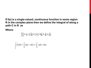


![RESIDUE THEORY
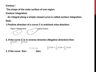
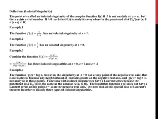
Definition (Residue)
Let f(z) has a non-removable isolated singularity at the point a
z0. Then f(z) has the Laurent series representation for all z in some
punctured disk DR
*(z0) given by 𝑓 𝑧 = 𝑛=−∞
∞
𝑎 𝑛 z − z0
𝑛
The coefficient a-1 of
1
𝑧−𝑧0
is called the residue of f(z) at z0 .
It is denoted by Res[f,z0] = a-1](https://image.slidesharecdn.com/complexintegration-200321125229/85/Complex-integration-25-320.jpg)
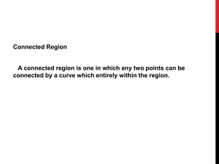
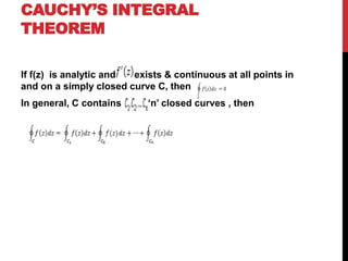
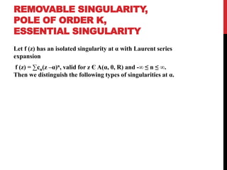
![Example.1
Consider f (z) = e2/z
Then the Laurent series of f about the point z0 = 0 is given by
= 1 +
2
1!z
+
22
2!z2 +
23
3!z3 + ⋯ ,
The co-efficient of
1
𝑧−𝑧0
=
1
𝑧−0
=
1
𝑧
is 2
Hence by definition of residue, residue of f (z) = e2/z at z0 = 0 is given by Res [f, z0] = 2
Example .2 Find residue of f (z) =
3
2𝑧+𝑧2−𝑧3 at z0 = 0
f(z) =
3
z 2+z−z2 =
3
z z+1 2−z
Now
3
z z+1 2−z
=
A
z
+
B
z+1
+
C
2−z
⇒A(z+1)(2-z) + Bz(2-z) + Cz (z+1) = 3
⇒A(-z2 +2 + z) +B(2z –z2) +C(z2 +z) = 3
⇒-A –B +C = 0---- (a)
A +2B +C = 0 ---- (b)
2A =3 ---- ( c) ⇒A = 3/2
(a) ⇒-B + C = A= 3/2
(b) ⇒2B + C = -A = -3/2
-----------------------------
Adding B + 2C =0⇒ B = - 2C
Put B = - 2C in -B + C = 3/2
⇒3C = 3/2⇒C= 1/2
Put C= 1/2, B = -2C = -1⇒ B = -1
Hence f(z) = =
A
z
+
B
z+1
+
C
2−z
=
3
2z
-
1
z+1
+
1
2(2−z)
=
3
2z
- (1+z) -1 +
1
2
(2-z)-1 =
3
2z
- (1- z+ z2 -….) +
1
2
2-1 =
3
2z
- (1- z+ z2 -….) +
1
4
(1 +
z
2
+
z
2
2
+ ….)
=
3
2z
-
3
4
+
9z
8
- …..
The residue of f at 0 is given by Res [f,0] = coefficient of
1
z
=
3
2
Example.3 Find residue of f (z) =
𝑒 𝑧
𝑧3 at z0 = 0
Laurent expansion of f(z) =
1
𝑧3 {1 + 𝑧 +
𝑧2
2!
+
𝑧3
3!
… } =
1
𝑧3 +
1
𝑧2 +
1
𝑧2!
+
1
3!
…
The residue of f at 0 is given by Res [f,0] = coefficient of
1
z
=
1
2](https://image.slidesharecdn.com/complexintegration-200321125229/85/Complex-integration-26-320.jpg)
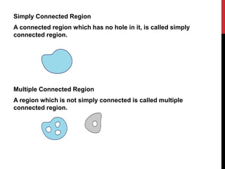
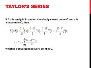
![CAUCHY'S RESIDUE
THEOREM
Let D be a simply connected domain, and let C ⊂D be a closed
positively oriented contour within and on the function f(z) is
analytic, except finite number of singular z1,z2,….,zn, then
𝐶
𝑓(𝑧) 𝑑𝑧 = 2πi 𝑘=1
𝑛
Res[f, zk]](https://image.slidesharecdn.com/complexintegration-200321125229/85/Complex-integration-27-320.jpg)
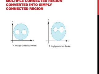
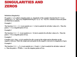
![Residues at Poles
(i) If f(z) has a simple pole at z0, then Res[f,z0] =
lim
𝑧 → 𝑧0
( 𝑧 −](https://image.slidesharecdn.com/complexintegration-200321125229/85/Complex-integration-28-320.jpg)
![Results
1. Let P(z) be a polynomial of degree at most 2. If a ,b and c are distinct complex
numbers,
then f(z) =
𝑃 𝑧
(𝑧−𝑎)(𝑧−𝑏)(𝑧−𝑐)
=
𝐴
(𝑧−𝑎)
+
𝐵
(𝑧−𝑏)
+
𝐶
(𝑧−𝑐)
Where A = Res [f,a] =
𝑃 𝑎
(𝑎−𝑏)(𝑎−𝑐)
B = Res [f,b] =
𝑃(𝑏)
(𝑏−𝑎)(𝑏−𝑐)
C = Res [f,c] =
𝑃(𝑐)
(𝑐−𝑎)(𝑐−𝑏)
2. If a repeated root occurs in partial fraction, and P(z) has degree of at most 2, then
f(z) =
𝑃 𝑧
𝑧−𝑎 2(𝑧−𝑏)
=
𝐴
𝑧−𝑎 2 +
𝐵
(𝑧−𝑎)
+
𝐶
(𝑧−𝑏)
Where A = Res [(z-a)f(z),a]
B = Res [f, a]
C = Res [f, b]](https://image.slidesharecdn.com/complexintegration-200321125229/85/Complex-integration-29-320.jpg)

![CASES OF POLES ARE NOT
ON THE REAL AXIS.
Type I
Evaluation of the integral 𝟎
𝟐𝝅
𝒇 𝒄𝒐𝒔𝜽𝒔𝒊𝒏𝜽 𝒅𝜽 where f(cosθsinθ) is a real rational function of
sinθ,cosθ.
First we use the transformation z = eiθ =cosθ + i sinθ ------ ( a)
And
1
𝑧
=
1
𝑒 𝑖𝜃 = e-iθ= cosθ - i sinθ -------- (b)
From (a) and (b) , we have cosθ =
1
2
(𝑧 +
1
𝑧
) , sinθ =
1
2𝑖
(𝑧 −
1
𝑧
)
Now z = eiθ⇒dz = ieiθdθ⇒dθ =
𝑑𝑧
𝑖𝑧
Hence 0
2𝜋
𝑓 𝑐𝑜𝑠𝜃𝑠𝑖𝑛𝜃 𝑑𝜃 = 𝐶
𝑓[
1
2
𝑧 +
1
𝑧
,
1
2𝑖
(𝑧 −
1
𝑧
)]
𝑑𝑧
𝑖𝑧
Where C, is the positively oriented unit circle |z| = 1
The LHS integral can be evaluated by the residue theorem and
𝐶
𝑓[
1
2
𝑧 +
1
𝑧
,
1
2𝑖
(𝑧 −
1
𝑧
)]
𝑑𝑧
𝑖𝑧
= 2πi ∑ Res(zi) , where zi is any pole in the interior of the
circle |z| =1](https://image.slidesharecdn.com/complexintegration-200321125229/85/Complex-integration-31-320.jpg)
![Type II.
Evaluation of the integral −∞
∞
𝒇 𝒙 𝒅𝒙 where f(x) is a real rational function of the real variable x.
If the rational function f(x) =
𝑔(𝑥)
ℎ(𝑥)
, then degree of h(x) exceeds that of g(x) and g(x) ≠ 0.To find the value of the
integral, by inventing a closed contour in the complex plane which includes the required integral. For this we have
to close the contour by a very large semi-circle in the upper half-plane. Suppose we use the symbol “R” for the
radius. The entire contour integral comprises the integral along the real axis from −R to +R together with the
integral along the semi-circular arc. In the limit as R→∞the contribution from the straight line part approaches
the required integral, while the curved section may in some cases vanish in the limit.
The poles z1,z2,….,zk of
𝑔(𝑥)
ℎ(𝑥)
, that lie in the upper half-plane
−∞
∞
𝑓 𝑥 𝑑𝑥 = −∞
∞ 𝑔(𝑥)
ℎ(𝑥)
𝑑𝑥= 2πi∑ Res[f,zk]](https://image.slidesharecdn.com/complexintegration-200321125229/85/Complex-integration-32-320.jpg)
![Type III.
Evaluation of the integral −∞
∞
𝒇 𝒙 𝒔𝒊𝒏 𝒎𝒙 𝒅𝒙 , −∞
∞
𝒇 𝒙 𝒄𝒐𝒔 𝒎𝒙 𝒅𝒙where m > 0 and f(x) is a real rational function of the
real variable x.
If the rational function f(x) =
𝑔(𝑥)
ℎ(𝑥)
, then degree of h(x) exceeds that of g(x) and g(x) ≠ 0.
Let g(x) and h(x) be polynomials with real coefficients, of degree p and q, respectively, where q ≥ p+1.
If h(x) ≠0 for all real x, and m is a real number satisfying m > 0, then
−∞
∞ 𝑔(𝑥)
ℎ(𝑥)
cos 𝑚𝑥 𝑑𝑥 = lim
𝑅→∞ −𝑅
𝑅 𝑔(𝑥)
ℎ(𝑥)
cos 𝑚𝑥 𝑑𝑥 and −∞
∞ 𝑔(𝑥)
ℎ(𝑥)
𝑠𝑖𝑛𝑚𝑥 𝑑𝑥 = lim
𝑅→∞ −𝑅
𝑅 𝑔(𝑥)
ℎ(𝑥)
sin 𝑚𝑥 𝑑𝑥
We know that Euler’s formula 𝑒 𝑖𝑚𝑥
= cos mx + i sin mx , where cos mx = Re[𝑒 𝑖𝑚𝑥
]
and sin mx = Im[𝑒 𝑖𝑚𝑥
] , m is a positive real.
We have −∞
∞ 𝑔(𝑥)
ℎ(𝑥)
𝑒 𝑖𝑚𝑥
𝑑𝑥 = −∞
∞ 𝑔(𝑥)
ℎ(𝑥)
cos 𝑚𝑥 𝑑𝑥 + i −∞
∞ 𝑔(𝑥)
ℎ(𝑥)
𝑠𝑖𝑛𝑚𝑥 𝑑𝑥
Here we are going to use the complex function f(z) =
𝑔(𝑧)
ℎ(𝑧)
𝑒 𝑖𝑚𝑧
to evaluate the given integral.
−∞
∞ 𝑔(𝑥)
ℎ(𝑥)
cos 𝑚𝑥 𝑑𝑥= Re{2πi∑ Res[f,zk]} and
−∞
∞ 𝑔(𝑥)
ℎ(𝑥)
𝑠𝑖𝑛𝑚𝑥 𝑑𝑥 = Im{2πi∑ Res[f,zk]}, where z1,z2,…..zk are the poles lies on the upper half of the semi-circle.](https://image.slidesharecdn.com/complexintegration-200321125229/85/Complex-integration-33-320.jpg)

![CASE OF POLES ARE ON THE REAL AXIS.
Type IV
If the rational function f(z) =
𝑔(𝑧)
ℎ(𝑧)
, then degree of h(z) exceeds that of g(z) and g(z) ≠ 0.
Suppose h(z) has simple zeros on the real axis ( that is simple poles of f(z) on the real axis) , let it be a1,a2,…ak
and h(z) has zeros inside the upper half of semi-circle ( that is poles of f(z) inside the upper half of semi-
circle), let it be b1,b2,…bs,
then −∞
∞
𝑓 𝑥 𝑑𝑥 = πi∑ Res[f,ak] + 2πi∑ Res[f,bs], where k = 1,2,….k and s = 1,2,…s
Where C1,C2,….Ck are the semi circles and b1,b2,…bs are lie upper half of these semi circles.](https://image.slidesharecdn.com/complexintegration-200321125229/85/Complex-integration-35-320.jpg)


The document outlines key concepts in complex analysis, including the definitions of connected, simply connected, and multiple connected regions, as well as contour integration and Cauchy's integral theorem. It discusses singularities and their classifications, such as removable singularities, poles, and essential singularities, with examples illustrating each type. Additionally, it presents Taylor and Laurent series expansions and their relevance to functions with singularities.


