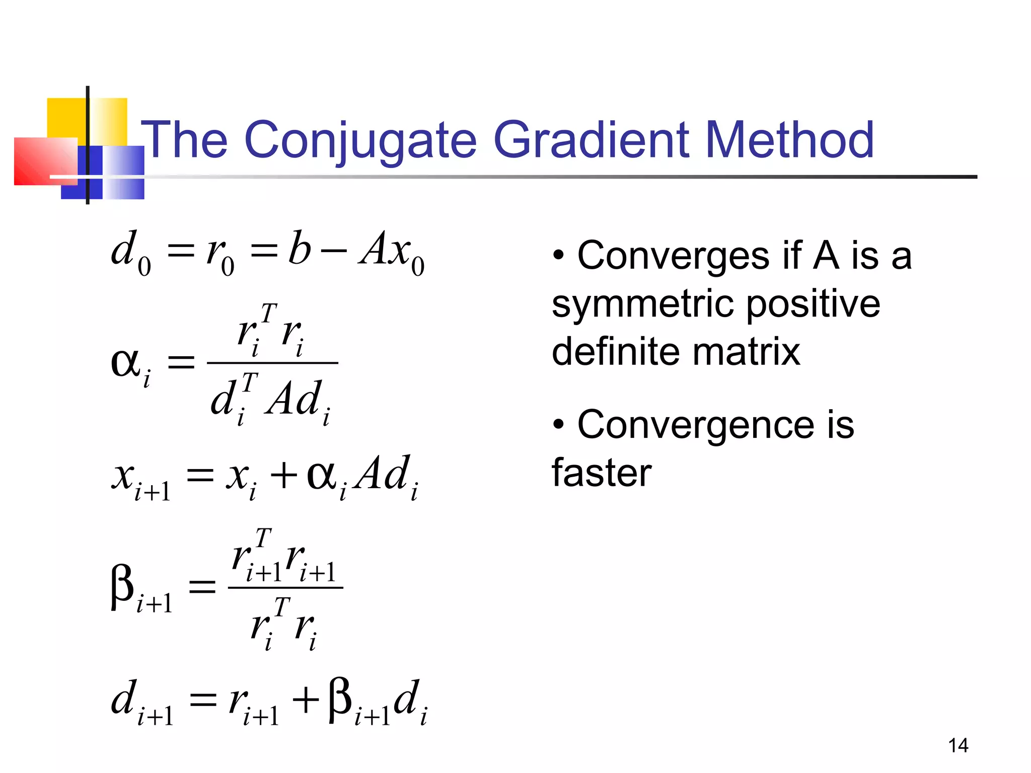
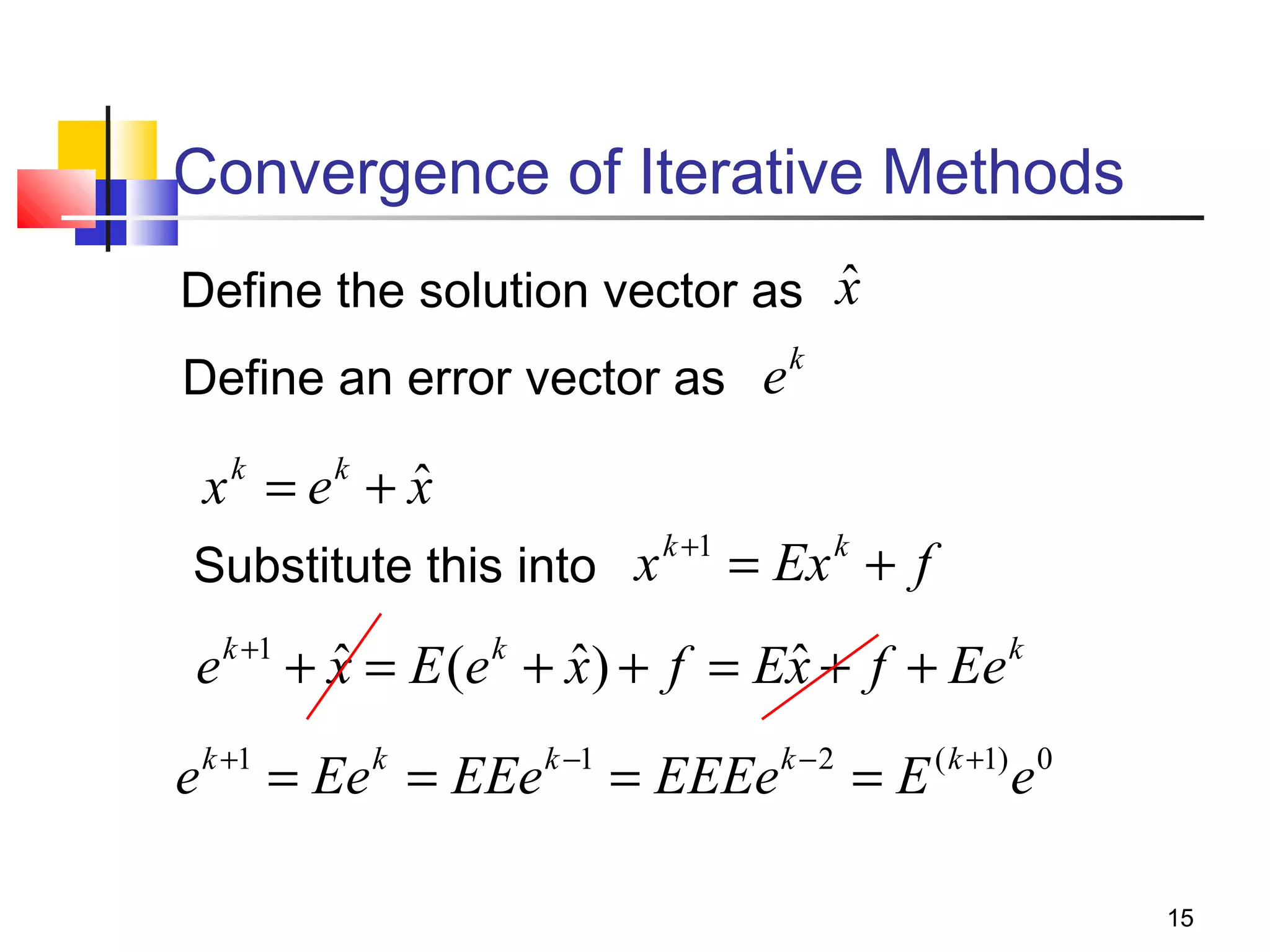
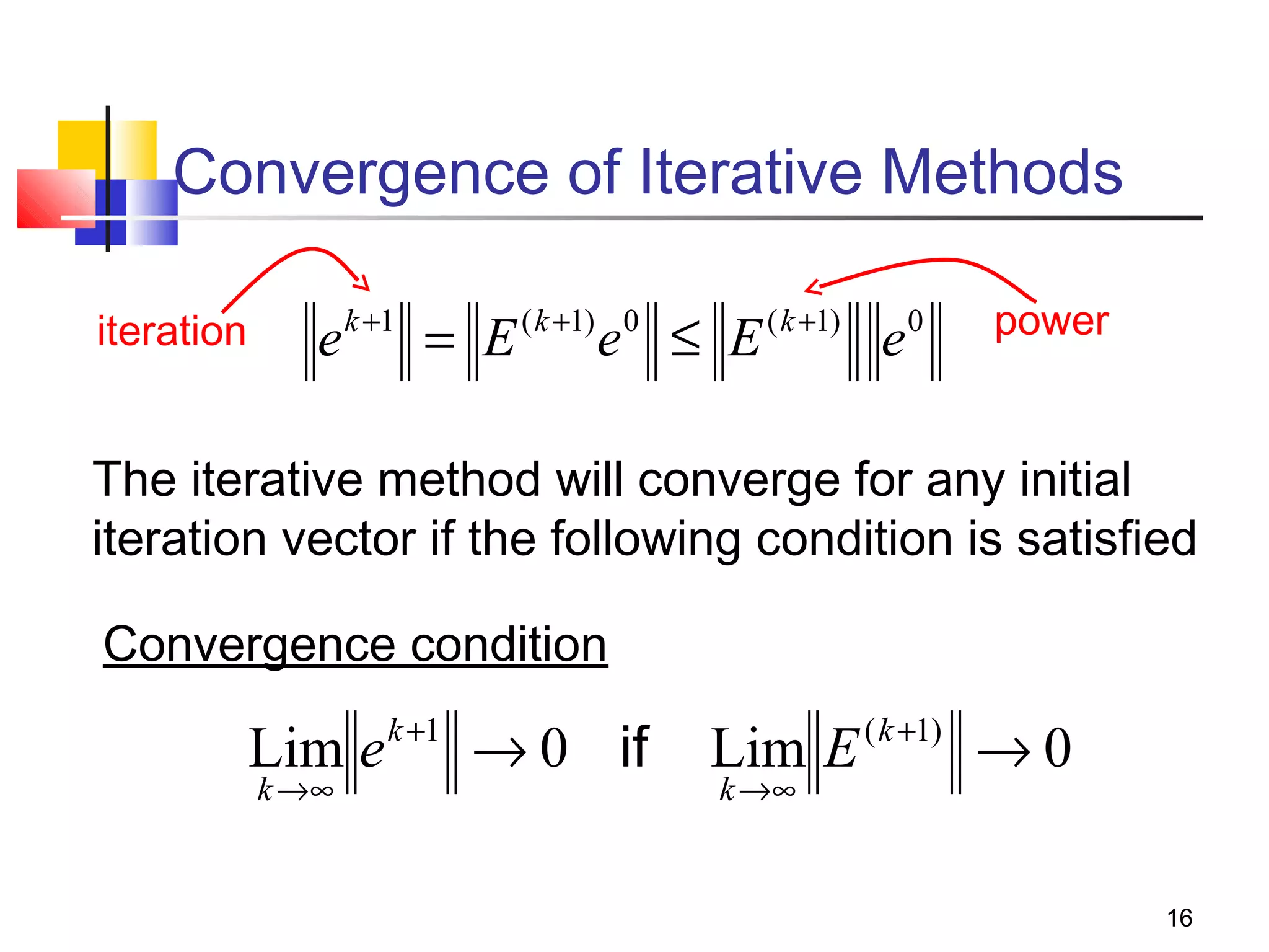
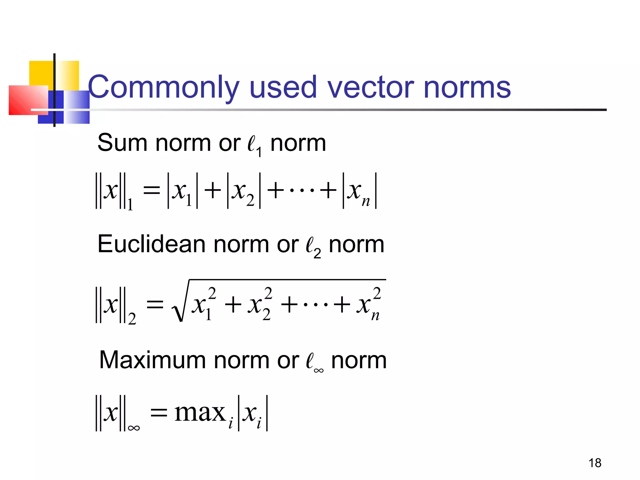
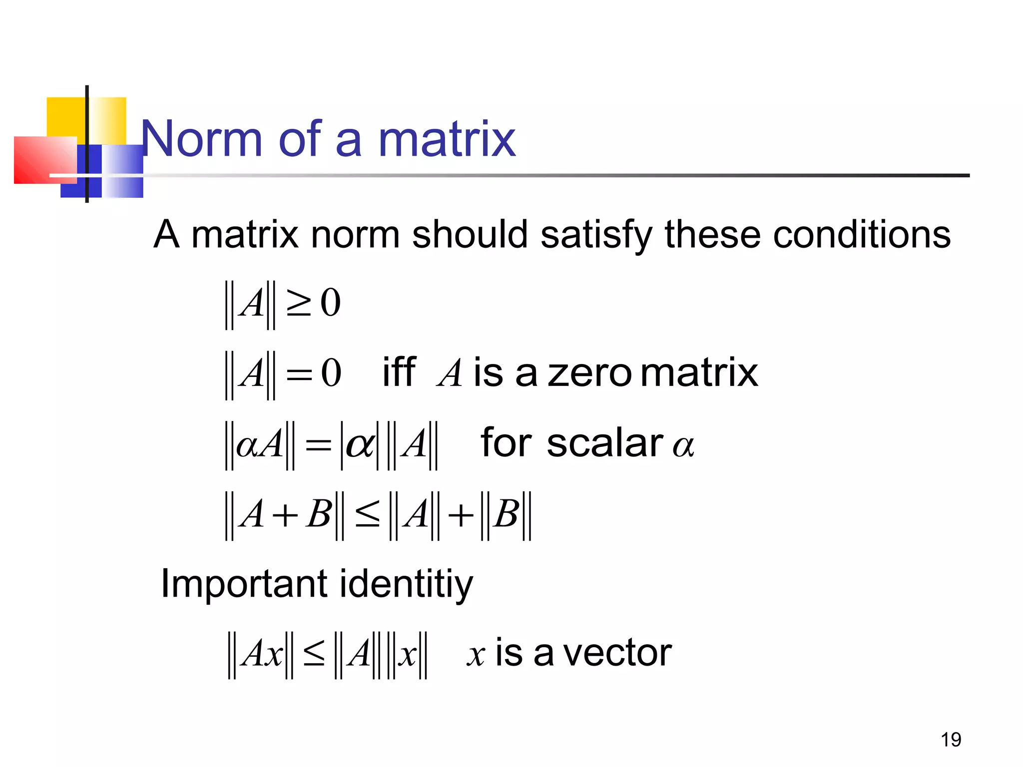
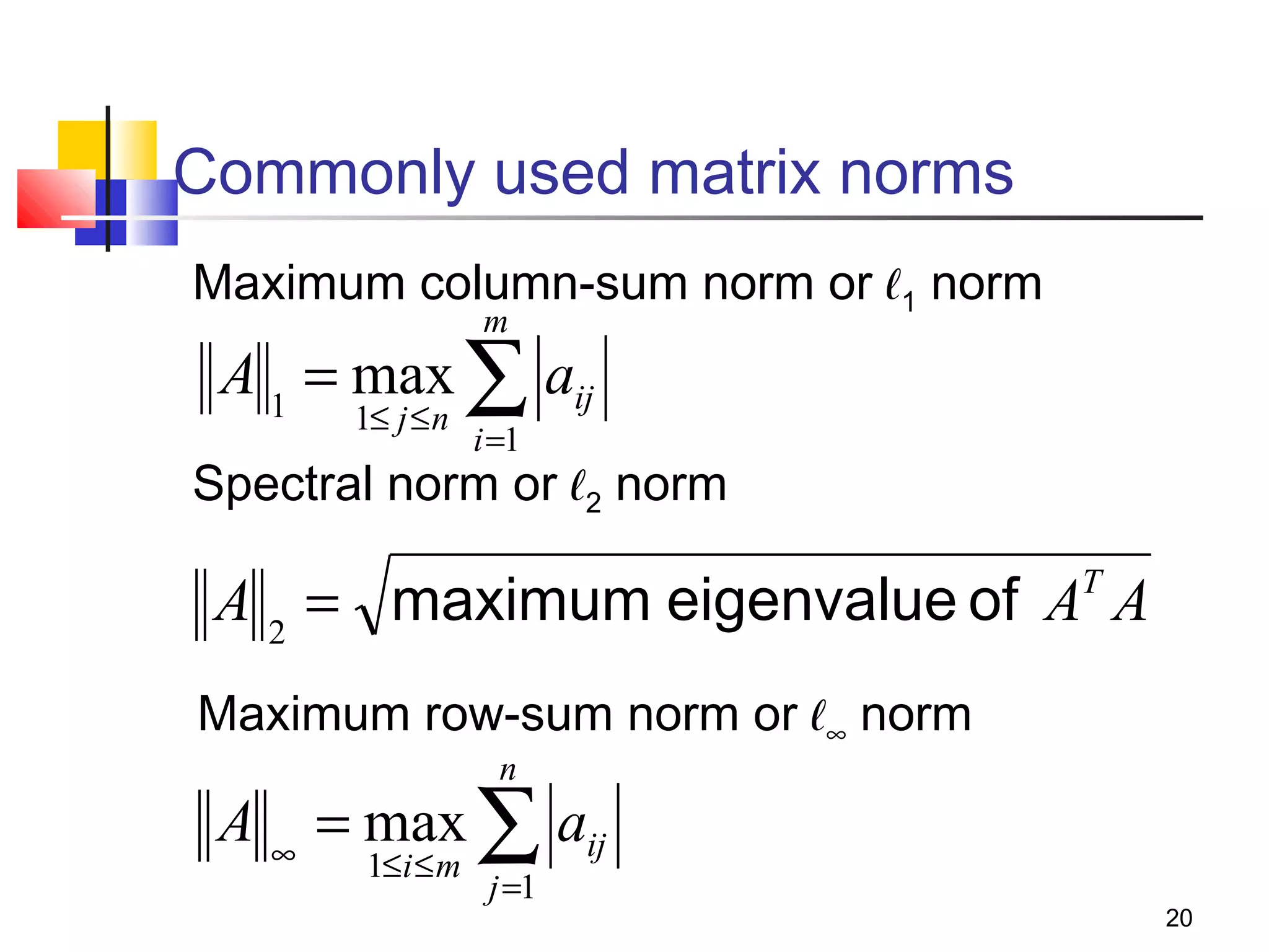
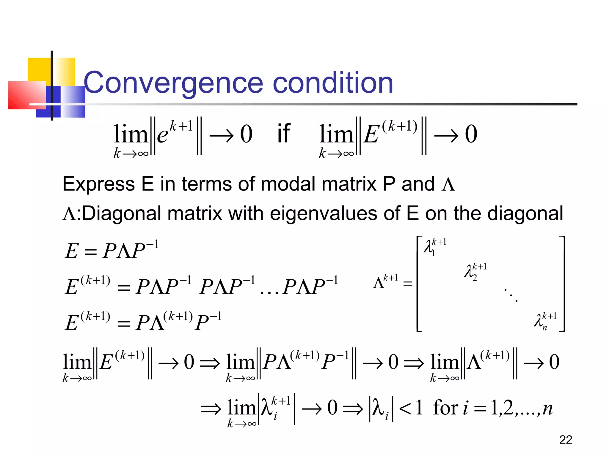
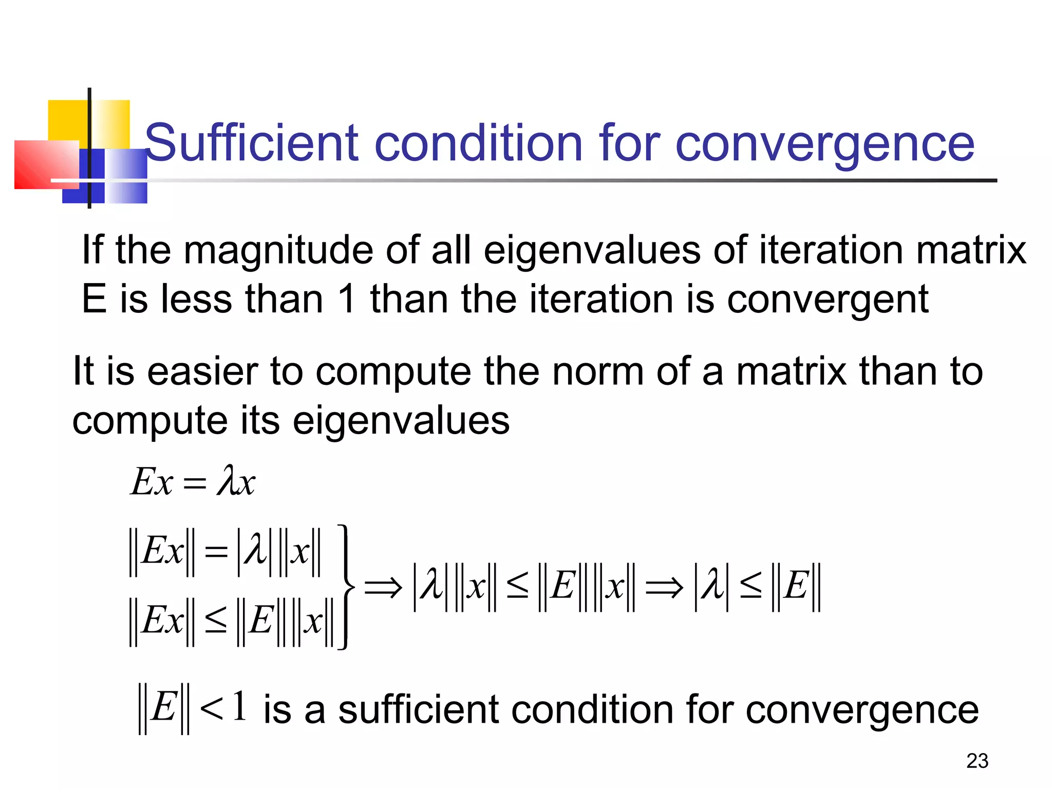
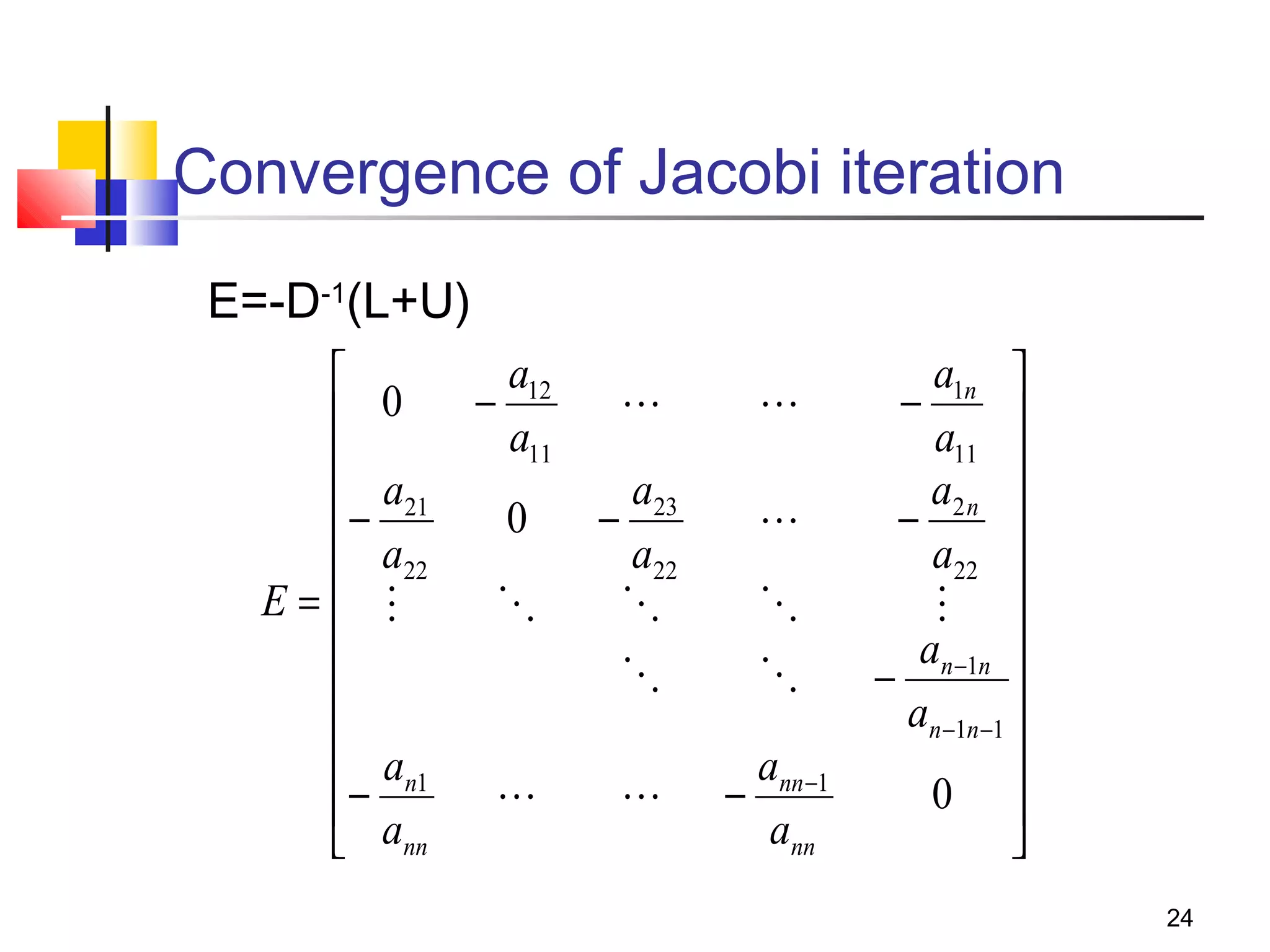
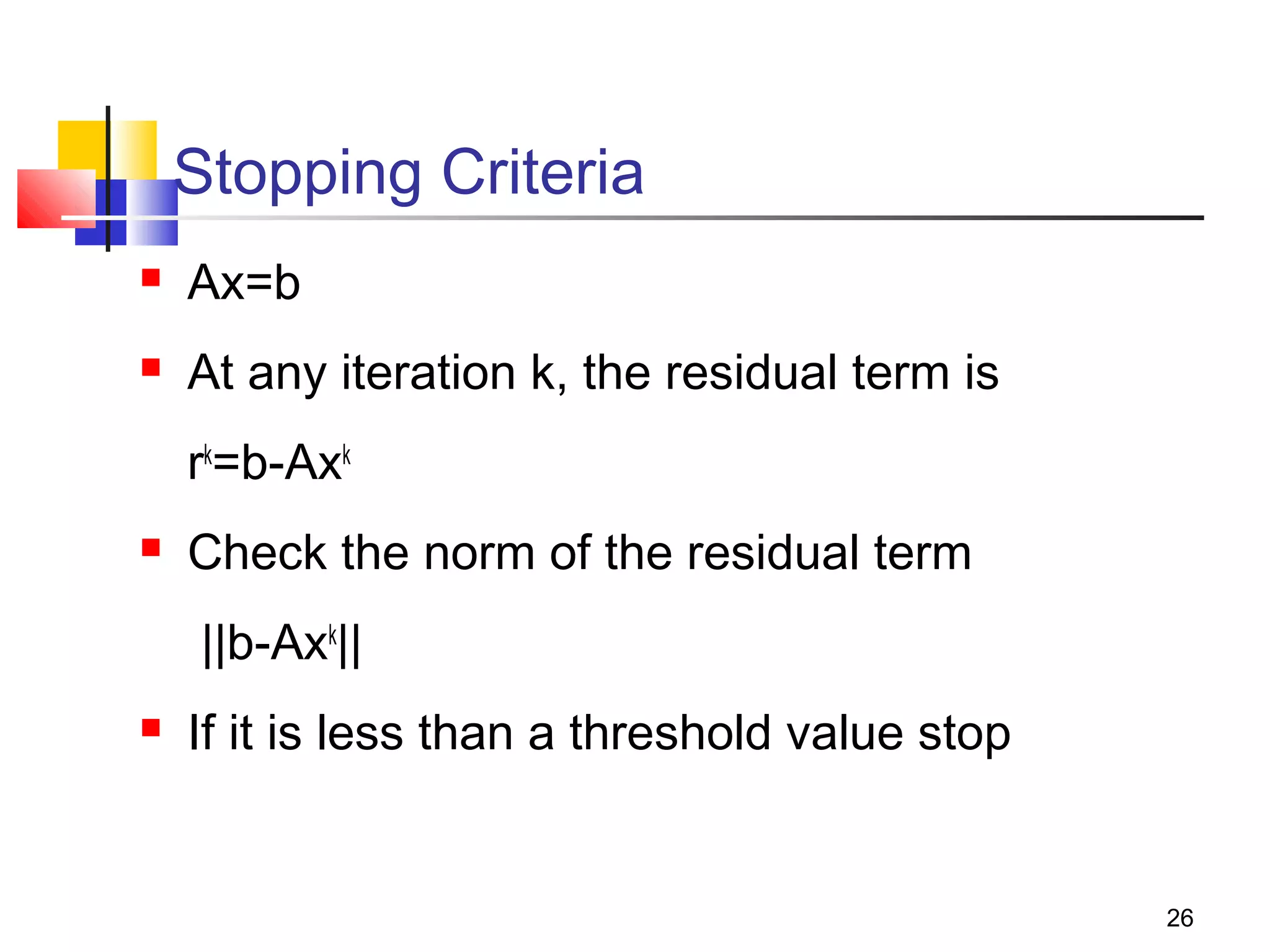
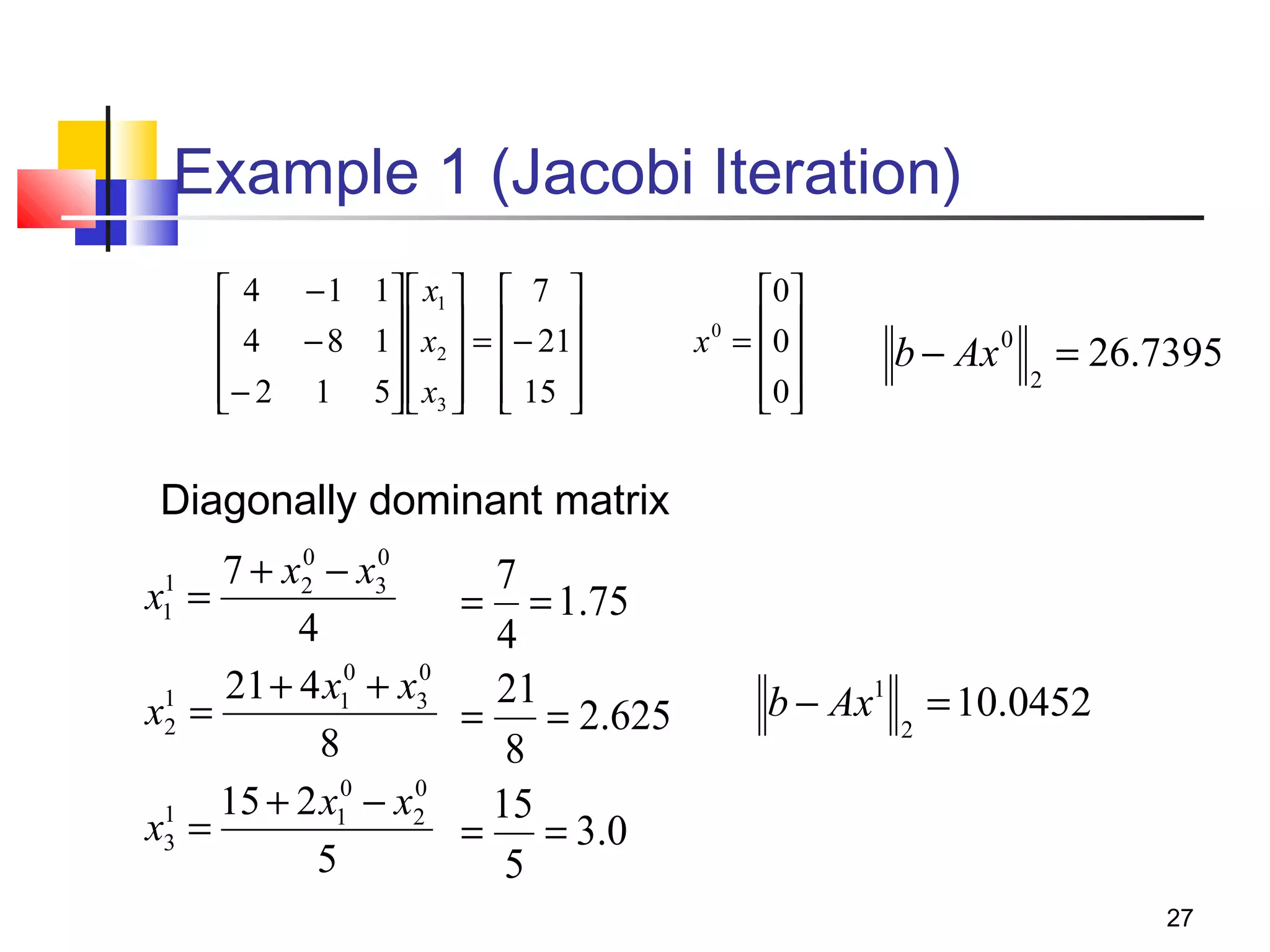
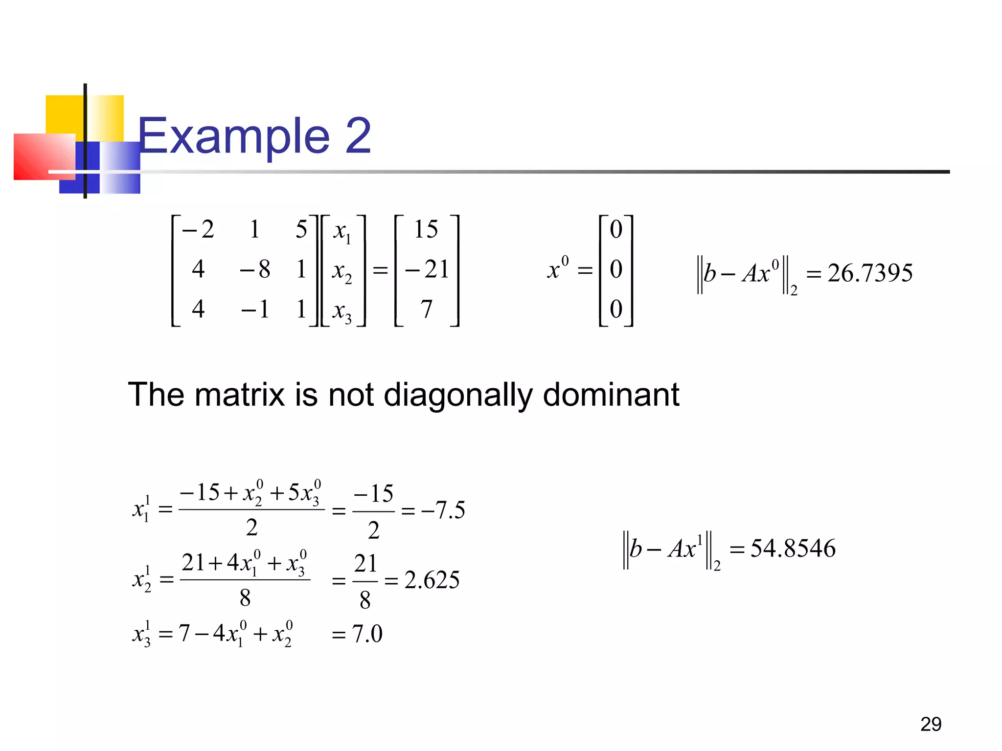
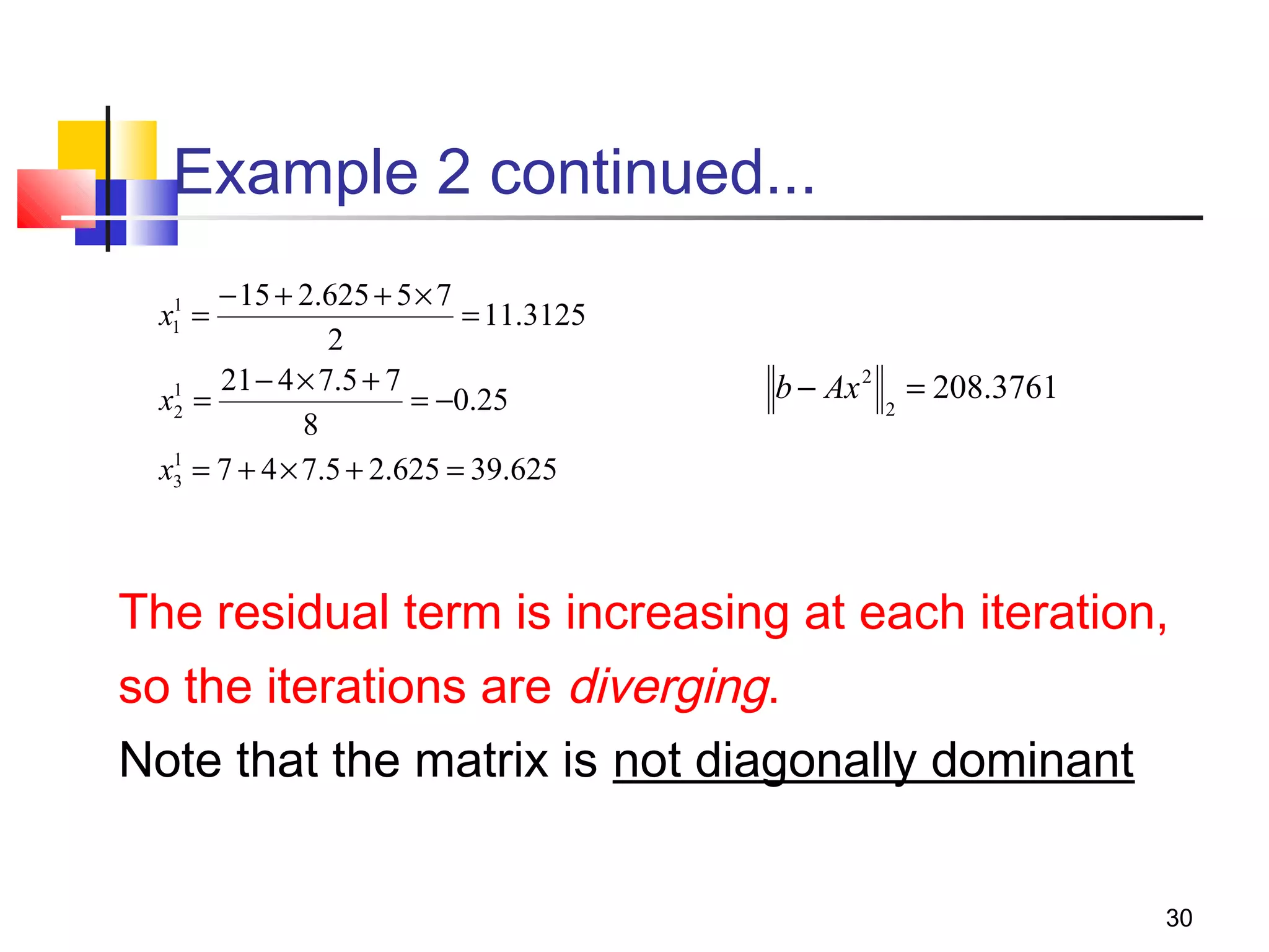
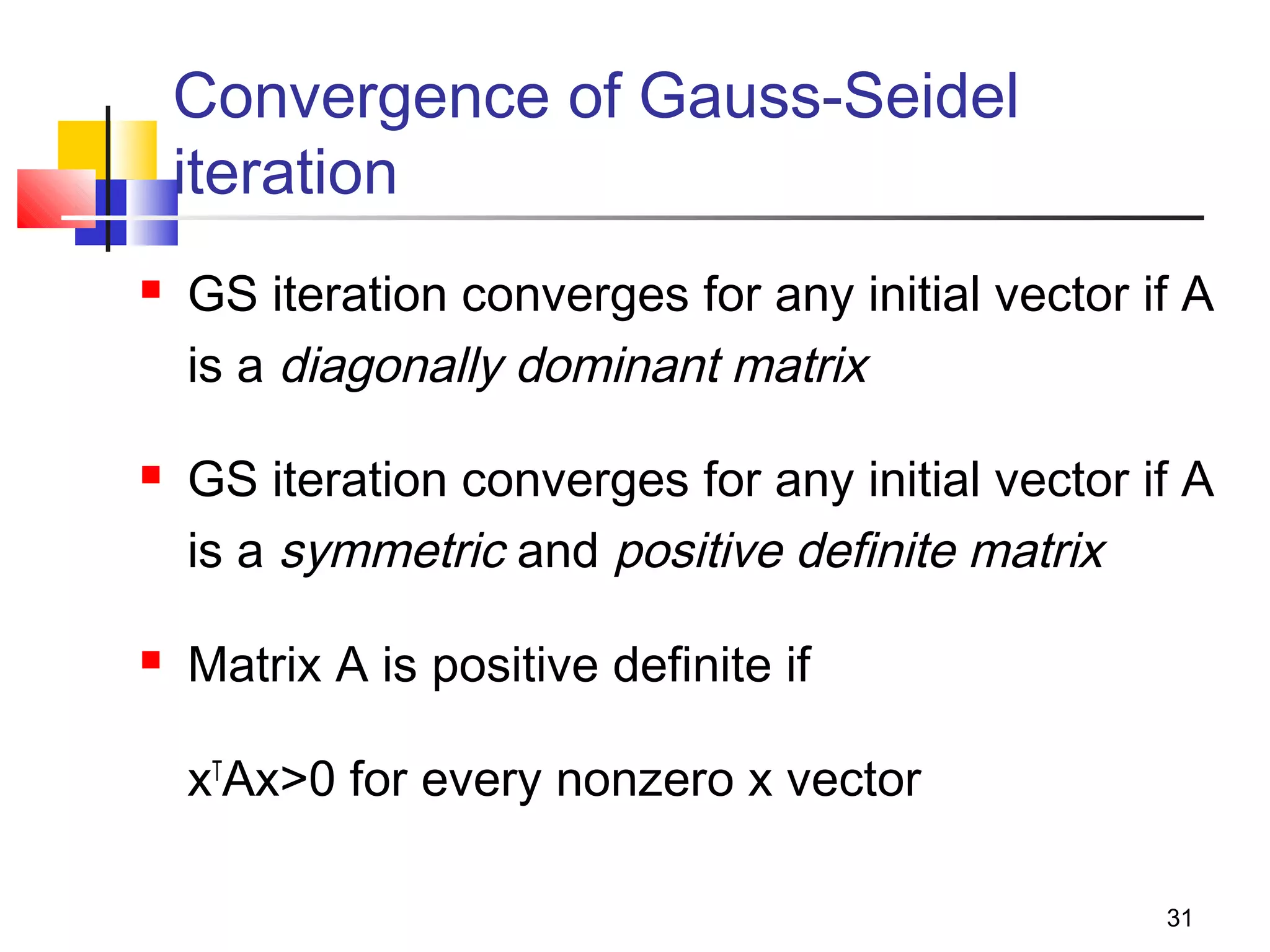
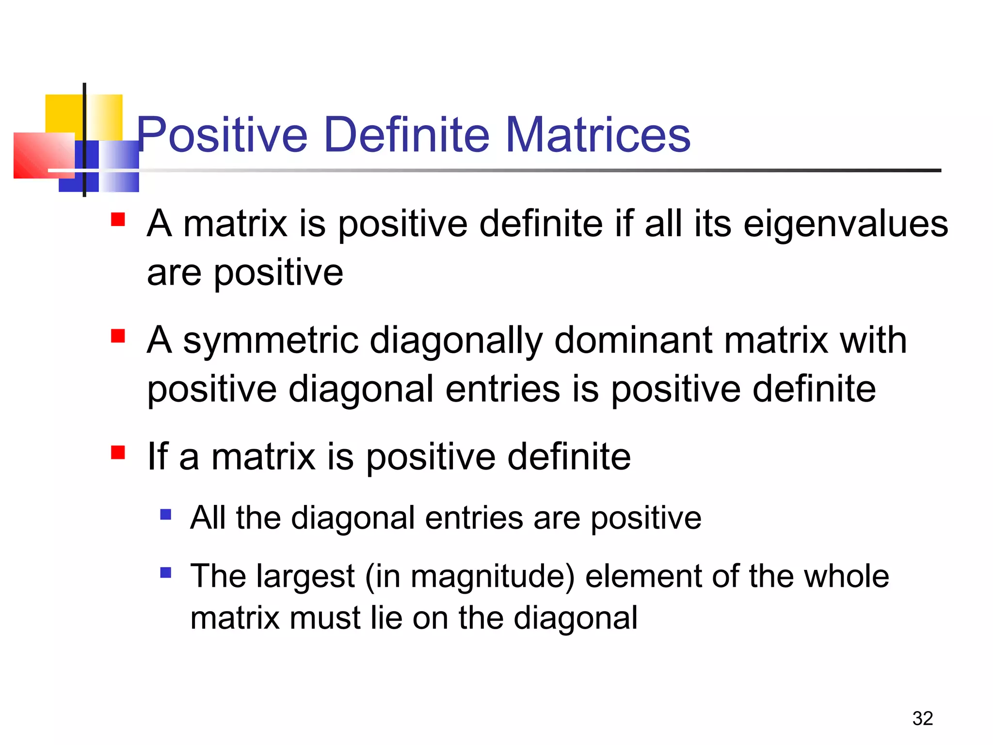
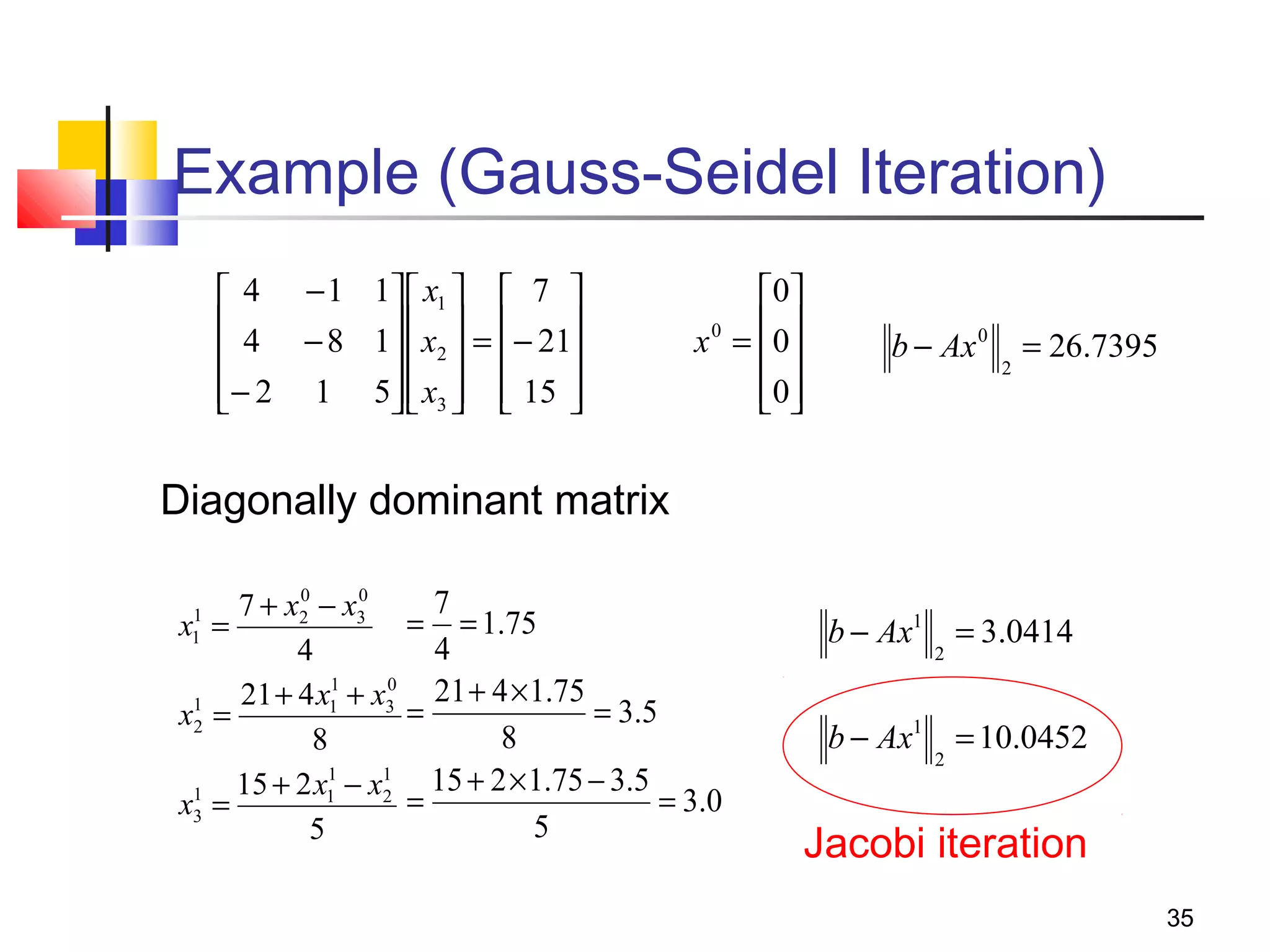
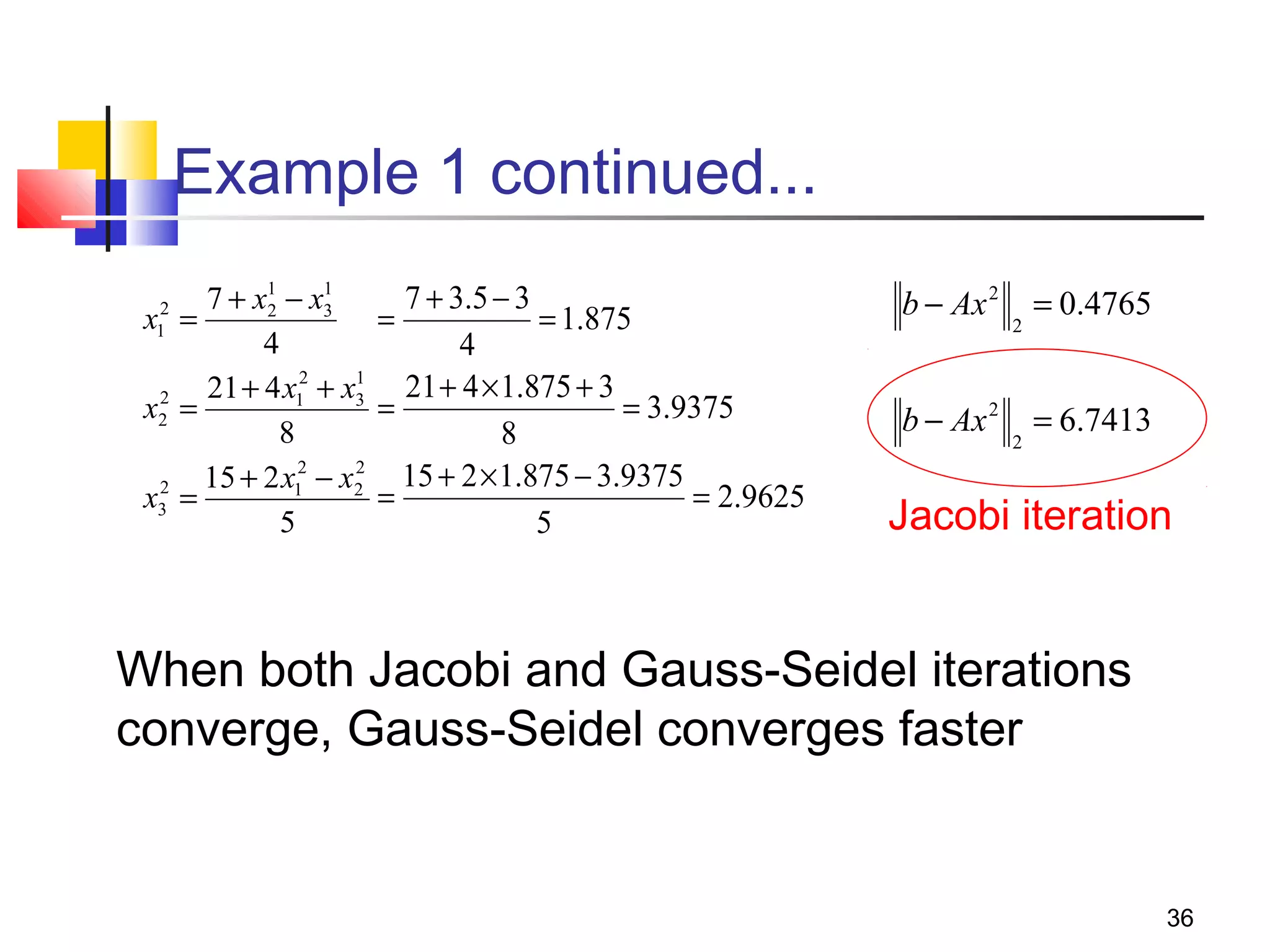
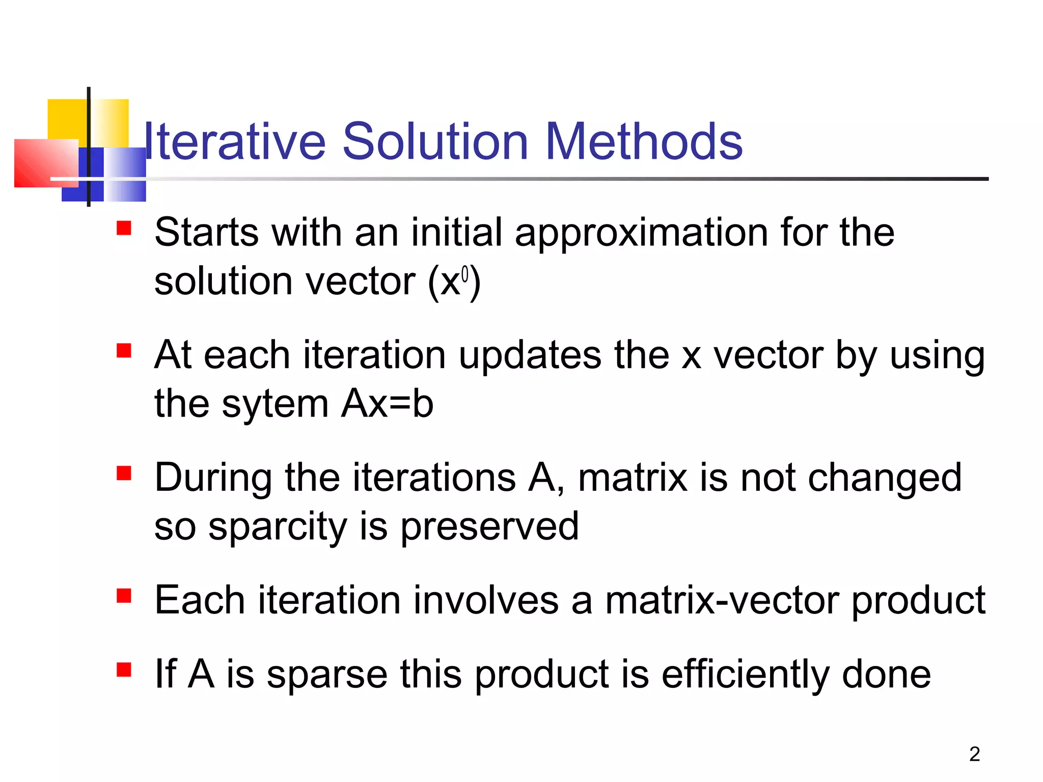
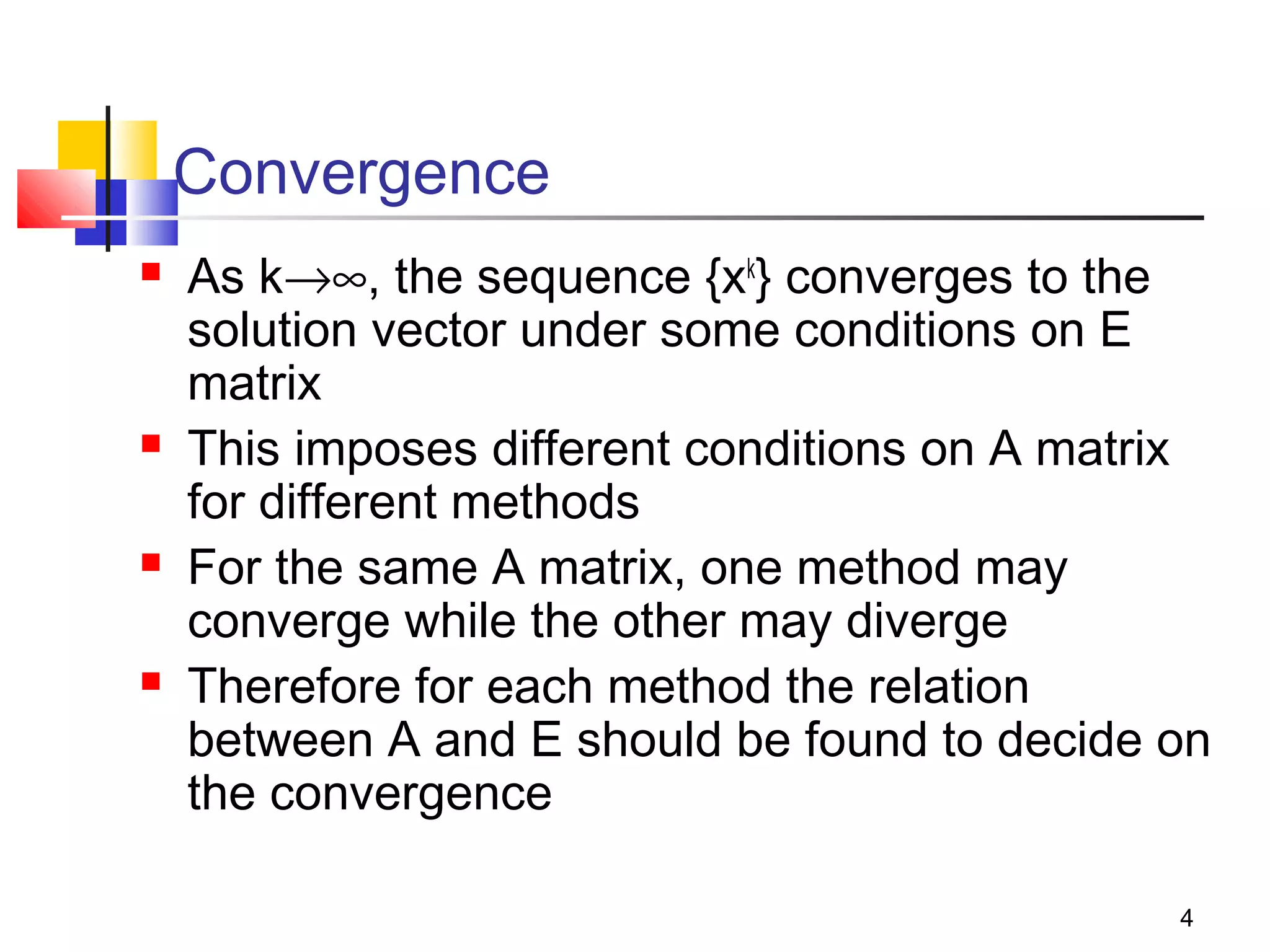
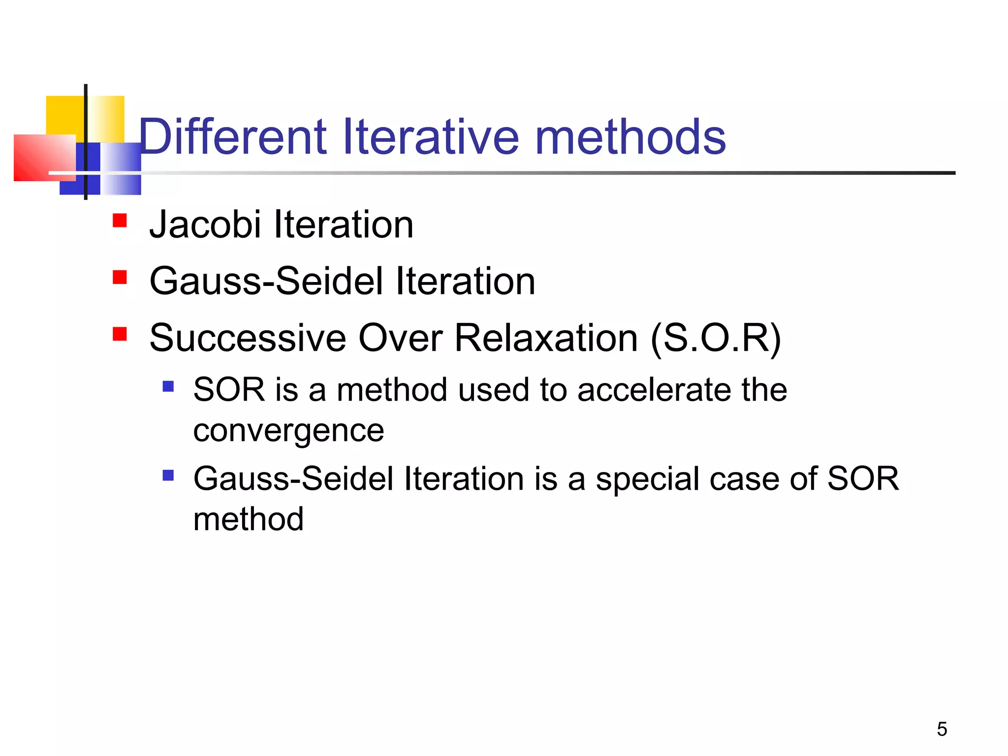
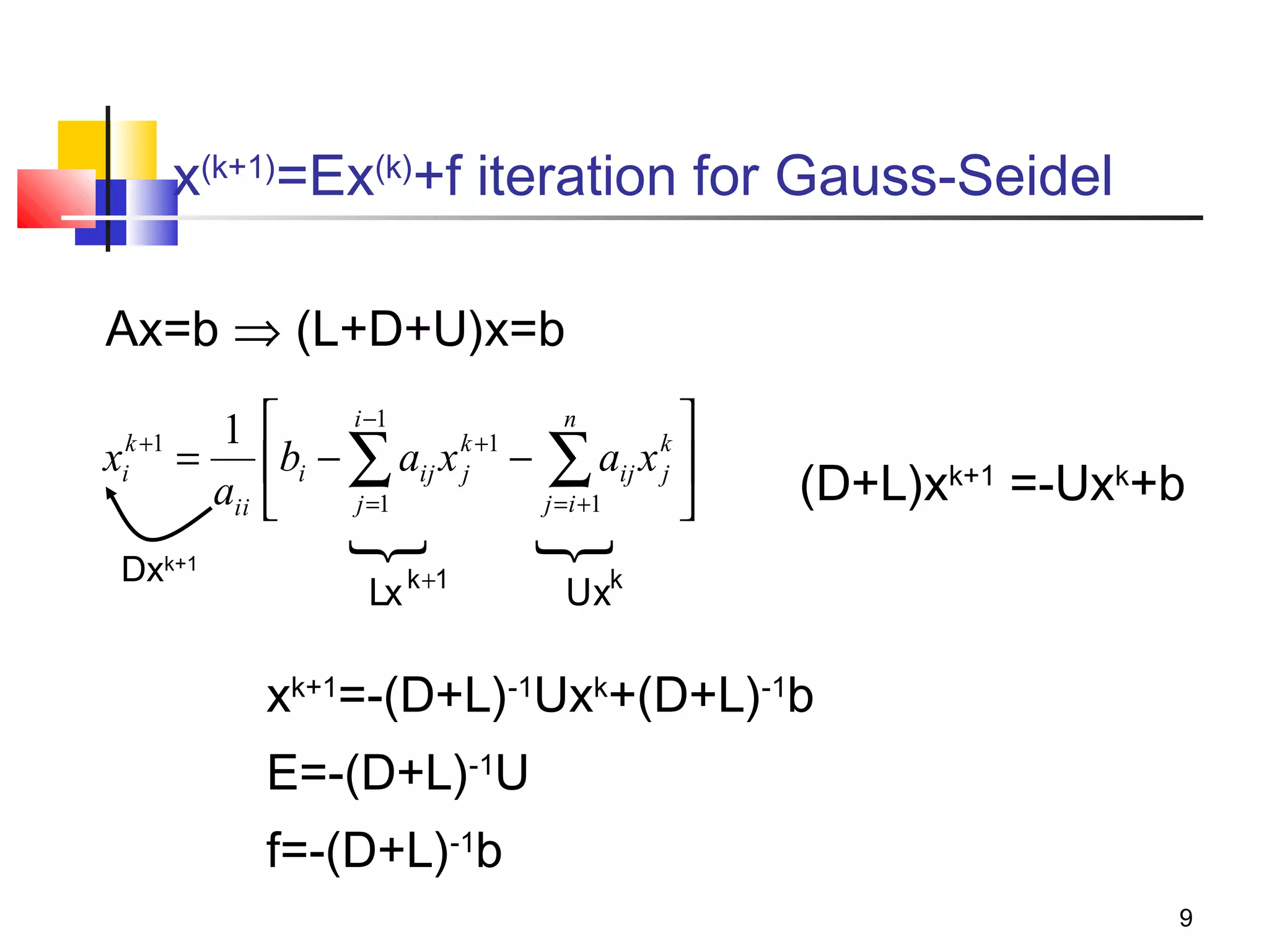
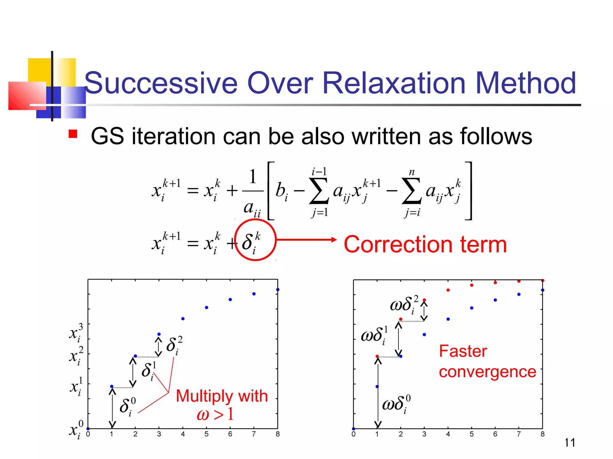
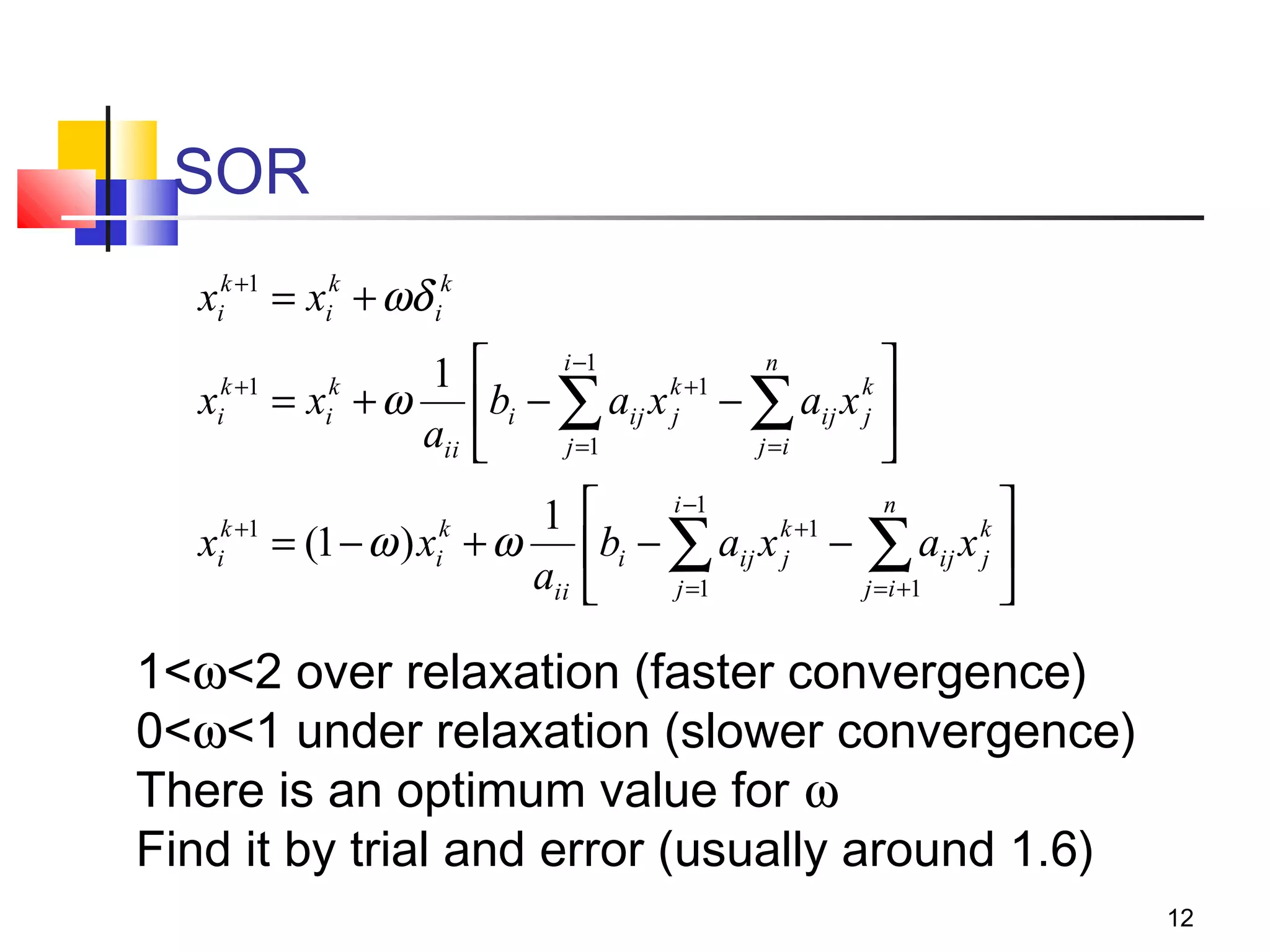
Iterative solution methods start with an initial approximation for the solution vector and iteratively update the vector at each step by using the system Ax=b. Different iterative methods like Jacobi, Gauss-Seidel, and Successive Over Relaxation represent the system in the form x=Ex+f and generate the next approximation. The iterative method converges if the spectral radius of E is less than 1 as the number of iterations increases. Different convergence criteria like the norm of the residual vector can be used to check when the iterations have converged to the solution.

1. Convergence Criteria
1

2. Iterative Solution Methods



Starts with an initial approximation for the
solution vector (x0)
At each iteration updates the x vector by using
the sytem Ax=b
During the iterations A, matrix is not changed
so sparcity is preserved

Each iteration involves a matrix-vector product

If A is sparse this product is efficiently done
2

3. Iterative solution procedure




Write the system Ax=b in an equivalent form
x=Ex+f (like x=g(x) for fixed-point iteration)
Starting with x0, generate a sequence of
approximations {xk} iteratively by
x k+1 =Ex k +f
Representation of E and f depends on the type
of the method used
But for every method E and f are obtained from
A and b, but in a different way
3

4. Convergence




As k→∞, the sequence {xk} converges to the
solution vector under some conditions on E
matrix
This imposes different conditions on A matrix
for different methods
For the same A matrix, one method may
converge while the other may diverge
Therefore for each method the relation
between A and E should be found to decide on
the convergence
4

5. Different Iterative methods



Jacobi Iteration
Gauss-Seidel Iteration
Successive Over Relaxation (S.O.R)


SOR is a method used to accelerate the
convergence
Gauss-Seidel Iteration is a special case of SOR
method
5

6. Jacobi iteration
a11 x1 + a12 x2 +  + a1n xn = b1
a21 x1 + a22 x2 +  + a2 n xn = b2

an1 x1 + an 2 x2 +  + ann xn = bn
 x10 
 0
0
 x2 
x =

 0
 xn 
 
1
0
0
1 
(b1 − a12 x2 −  − a1n xn )
k +1
xi = bi −
a11
aii 
1
0
0
x1 =
(b2 − a21 x10 − a23 x3 −  − a2 n xn )
2
a22
1
0
0
x1 =
(bn − an1 x10 − an 2 x2 −  − ann −1 xn −1 )
n
ann
1
x1 =

∑ aij x − j∑1aij x 
j =1
=i +

i −1
k
j
n
k
j
6

7. xk+1=Exk+f iteration for Jacobi method
A can be written as A=L+D+U (not decomposition)
0 0  a11 0
0  0 a12 a13 
 a11 a12 a13   0
a
a22 a23  =  a21 0 0 +  0 a22 0  + 0 0 a23 
 21
 
 
 

 a31 a32 a33   a31 a32 0  0
0 a33  0 0
0

 
 
 

Ax=b ⇒ (L+D+U)x=b
1
k +1
xi =
aii
Dxk+1
i −1
n


k
k
bi − ∑ aij x j − ∑ aij x j 
j =1
j = i +1



Lx k

Uxk
Dxk+1 =-(L+U)xk+b
xk+1=-D-1(L+U)xk+D-1b
E=-D-1(L+U)
f=D-1b
7

8. Gauss-Seidel (GS) iteration
Use the latest
update
a11 x1 + a12 x2 +  + a1n xn = b1
a21 x1 + a22 x2 +  + a2 n xn = b2

an1 x1 + an 2 x2 +  + ann xn = bn
1
0
0
1 
(b1 − a12 x2 −  − a1n xn )
k +1
xi = bi −
a11
aii 
1
1
1
0
0
x2 =
(b2 − a21 x1 − a23 x3 −  − a2 n xn )
a22
1
1
x1 =
(bn − an1 x1 − an 2 x1 −  − ann −1 x1 −1 )
n
2
n
ann
1
x1 =
 x10 
 0
0
 x2 
x =

 0
 xn 
 
i −1
∑a x
j =1
ij
k +1
j

− ∑ aij x 
j = i +1

n
k
j
8

9. x(k+1)=Ex(k)+f iteration for Gauss-Seidel
Ax=b ⇒ (L+D+U)x=b
k +1
i
x
Dx
1
=
aii
k+1
i −1
n


k +1
k
bi − ∑ aij x j − ∑ aij x j 
j =1
j = i +1



Lx k +1

(D+L)xk+1 =-Uxk+b
Uxk
xk+1=-(D+L)-1Uxk+(D+L)-1b
E=-(D+L)-1U
f=-(D+L)-1b
9

10. Comparison



Gauss-Seidel iteration converges more rapidly
than the Jacobi iteration since it uses the latest
updates
But there are some cases that Jacobi iteration
does converge but Gauss-Seidel does not
To accelerate the Gauss-Seidel method even
further, successive over relaxation method can
be used
10

11. Successive Over Relaxation Method

GS iteration can be also written as follows
k +1
i
x
1
=x +
aii
k
i
i −1
n


k +1
k
bi − ∑ aij x j − ∑ aij x j 
j =1
j =i


xik +1 = xik + δ ik
Correction term
ωδ i2
xi3
xi2
xi1
0
i
x
δ
ωδ i1
2
i
δ i1
δ i0
Multiply with
ω >1
Faster
convergence
ωδ i0
11

12. SOR
xik +1 = xik + ωδ ik
i −1
n


k +1
k
x
bi − ∑ aij x j − ∑ aij x j 
j =1
j =i


i −1
n

1 
k +1
k
k +1
k
xi = (1 − ω ) xi + ω bi − ∑ aij x j − ∑ aij x j 
aii 
j =1
j =i +1

k +1
i
1
= x +ω
aii
k
i
1<ω<2 over relaxation (faster convergence)
0<ω<1 under relaxation (slower convergence)
There is an optimum value for ω
Find it by trial and error (usually around 1.6)
12

13. x(k+1)=Ex(k)+f iteration for SOR
1
k +1
k
xi = (1 − ω ) xi + ω
aii
i −1
n


k +1
k
bi − ∑ aij x j − ∑ aij x j 
j =1
j = i +1


Dxk+1=(1-ω)Dxk+ωb-ωLxk+1-ωUxk
(D+ ωL)xk+1=[(1-ω)D-ωU]xk+ωb
E=(D+ ωL)-1[(1-ω)D-ωU]
f= ω(D+ ωL)-1b
13

14. The Conjugate Gradient Method
d 0 = r0 = b − Ax0
T
ri ri
αi = T
d i Ad i
xi +1 = xi + α i Ad i
• Converges if A is a
symmetric positive
definite matrix
• Convergence is
faster
T
i +1 i +1
T
i i
r r
βi +1 =
r r
d i +1 = ri +1 + βi +1d i
14

15. Convergence of Iterative Methods
ˆ
Define the solution vector as x
k
Define an error vector as e
ˆ
x =e +x
k
k
Substitute this into x
k +1
= Ex + f
k
ˆ
ˆ
ˆ
e k +1 + x = E (e k + x) + f = Ex + f + Ee k
e k +1 = Ee k = EEe k −1 = EEEe k − 2 = E ( k +1) e 0
15

16. Convergence of Iterative Methods
iteration
e
k +1
= E
( k +1) 0
e ≤ E
( k +1)
e
0
power
The iterative method will converge for any initial
iteration vector if the following condition is satisfied
Convergence condition
Lim e k +1 → 0 if
k →∞
Lim E ( k +1) → 0
k →∞
16

17. Norm of a vector
A vector norm should satisfy these conditions
x ≥ 0 for every nonzero vector x
x = 0 iff x is a zero vector
αx = α x
for scalar α
x+ y ≤ x + y
Vector norms can be defined in different forms as
long as the norm definition satisfies these conditions
17

18. Commonly used vector norms
Sum norm or ℓ1 norm
x 1 = x1 + x2 +  + xn
Euclidean norm or ℓ2 norm
2
2
x 2 = x12 + x2 +  + xn
Maximum norm or ℓ∞ norm
x
∞
= max i xi
18

19. Norm of a matrix
A matrix norm should satisfy these conditions
A ≥0
A = 0 iff A is a zero matrix
for scalar α
αA = α A
A+ B ≤ A + B
Important identitiy
Ax ≤ A x
x is a vector
19

20. Commonly used matrix norms
Maximum column-sum norm or ℓ1 norm
m
A 1 = max ∑ aij
1≤ j ≤ n
i =1
Spectral norm or ℓ2 norm
A 2 = maximum eigenvalue of AT A
Maximum row-sum norm or ℓ∞ norm
n
A ∞ = max ∑ aij
1≤i ≤ m
j =1
20

21. Example

Compute the ℓ1 and ℓ∞ norms of the matrix
3 9 5
7 2 4 


6 8 1 


16
19
17 = A ∞
13
15
10
= A1
21

22. Convergence condition
lim e
k →∞
k +1
→ 0 if
lim E
k →∞
( k +1)
→0
Express E in terms of modal matrix P and Λ
Λ:Diagonal matrix with eigenvalues of E on the diagonal
E = PΛP
−1
E ( k +1) = PΛP −1 PΛP −1  PΛP −1
E ( k +1) = PΛ( k +1) P −1
k
λ1 +1



λk +1
2

Λk +1 = 





λk +1 

n 

lim E ( k +1) → 0 ⇒ lim PΛ( k +1) P −1 → 0 ⇒ lim Λ( k +1) → 0
k →∞
k →∞
k →∞
⇒ lim λki +1 → 0 ⇒ λ i < 1 for i = 1,2 ,...,n
k →∞
22

23. Sufficient condition for convergence
If the magnitude of all eigenvalues of iteration matrix
E is less than 1 than the iteration is convergent
It is easier to compute the norm of a matrix than to
compute its eigenvalues
Ex = λx
Ex = λ x 

⇒ λ x ≤ E x ⇒ λ ≤ E
Ex ≤ E x 

E < 1 is a sufficient condition for convergence
23

24. Convergence of Jacobi iteration
E=-D-1(L+U)

 0

 − a21
 a22
E= 



 an1
− a
 nn
a12
−
a11
0


a23
−
a22








ann −1
−
ann
a1n 
−
a11 

a2 n 
−
a22 
 
an −1n 
−

an −1n −1 

0 

24

25. Convergence of Jacobi iteration
Evaluate the infinity(maximum row sum) norm of E
E
n
∞
<1⇒ ∑
j =1
i≠ j
aij
< 1 for i = 1,2,..., n
aii
n
⇒ aii > ∑ aij
j =1
i≠ j
Diagonally dominant matrix
If A is a diagonally dominant matrix, then Jacobi
iteration converges for any initial vector
25

26. Stopping Criteria

Ax=b

At any iteration k, the residual term is
rk=b-Axk

Check the norm of the residual term
||b-Axk||

If it is less than a threshold value stop
26

27. Example 1 (Jacobi Iteration)
 4 − 1 1  x1   7 
 4 − 8 1  x  = − 21

 2  

− 2 1 5  x3   15 

  

0 
x 0 = 0 
 
0 
 
b − Ax 0
2
= 26.7395
Diagonally dominant matrix
0
0
7 + x2 − x3
7
x =
= = 1.75
4
4
0
21 + 4 x10 + x3
21
x1 =
= = 2.625
2
8
8
0
15 + 2 x10 − x2
15
1
x3 =
= = 3.0
5
5
1
1
b − Ax1 = 10.0452
2
27

28. Example 1 continued...
1
7 + x1 − x3
7 + 2.625 − 3
2
x =
=
= 1.65625
4
4
1
1
21 + 4 x1 + x3 21 + 4 × 1.75 + 3
2
x2 =
=
= 3.875
8
8
1
15 + 2 x1 − x1 15 + 2 × 1.75 − 2.625
2
2
=
= 4.225
x3 =
5
5
2
1
7 + 3.875 − 4.225
= 1.6625
4
21 + 4 ×1.65625 + 4.225
3
x2 =
= 3.98125
8
15 + 2 × 1.65625 − 3.875
3
x3 =
= 2.8875
5
b − Ax 2
2
= 6.7413
x13 =
b − Ax 2
2
= 1.9534
Matrix is diagonally dominant, Jacobi iterations are converging
28

29. Example 2
− 2 1 5  x1   15 
 4 − 8 1  x  = − 21

 2  

 4 − 1 1  x3   7 

  

0 
x 0 = 0 
 
0 
 
b − Ax 0
2
= 26.7395
The matrix is not diagonally dominant
0
0
− 15 + x2 + 5 x3 − 15
x =
=
= −7.5
2
2
0
21 + 4 x10 + x3
21
1
x2 =
= = 2.625
8
8
1
0
x3 = 7 − 4 x10 + x2
= 7.0
1
1
b − Ax1 = 54.8546
2
29

30. Example 2 continued...
− 15 + 2.625 + 5 × 7
= 11.3125
2
21 − 4 × 7.5 + 7
x1 =
= −0.25
2
8
1
x3 = 7 + 4 × 7.5 + 2.625 = 39.625
1
x1 =
b − Ax 2
2
= 208.3761
The residual term is increasing at each iteration,
so the iterations are diverging.
Note that the matrix is not diagonally dominant
30

31. Convergence of Gauss-Seidel
iteration



GS iteration converges for any initial vector if A
is a diagonally dominant matrix
GS iteration converges for any initial vector if A
is a symmetric and positive definite matrix
Matrix A is positive definite if
xTAx>0 for every nonzero x vector
31

32. Positive Definite Matrices



A matrix is positive definite if all its eigenvalues
are positive
A symmetric diagonally dominant matrix with
positive diagonal entries is positive definite
If a matrix is positive definite


All the diagonal entries are positive
The largest (in magnitude) element of the whole
matrix must lie on the diagonal
32

33. Positive Definitiness Check
20 12 25
12 15 2 


 25 2 5 


Not positive definite
Largest element is not on the diagonal
5
20 12
12 − 15 2 


5
2 25


Not positive definite
All diagonal entries are not positive
20 12 5 
12 15 2 


 5 2 25


Positive definite
Symmetric, diagonally dominant, all
diagonal entries are positive
33

34. Positive Definitiness Check
20 12 5 
12 15 2 


 8 2 25


A decision can not be made just by investigating
the matrix.
The matrix is diagonally dominant and all diagonal
entries are positive but it is not symmetric.
To decide, check if all the eigenvalues are positive
34

35. Example (Gauss-Seidel Iteration)
 4 − 1 1  x1   7 
 4 − 8 1  x  = − 21

 2  

− 2 1 5  x3   15 

  

0 
x 0 = 0 
 
0 
 
b − Ax 0
2
= 26.7395
Diagonally dominant matrix
0
0
7
7 + x2 − x3
= = 1.75
x =
4
4
1
0
21 + 4 x1 + x3 21 + 4 × 1.75
1
=
= 3 .5
x2 =
8
8
1
15 + 2 x1 − x1 15 + 2 × 1.75 − 3.5
1
2 =
= 3 .0
x3 =
5
5
1
1
b − Ax1 = 3.0414
2
b − Ax1 = 10.0452
2
Jacobi iteration
35

36. Example 1 continued...
1
7 + 3.5 − 3
7 + x1 − x3
2
x =
=
= 1.875
4
4
1
21 + 4 x12 + x3 21 + 4 × 1.875 + 3
2
x2 =
=
= 3.9375
8
8
2
15 + 2 x12 − x2 15 + 2 × 1.875 − 3.9375
2
=
= 2.9625
x3 =
5
5
2
1
b − Ax 2
b − Ax 2
2
2
= 0.4765
= 6.7413
Jacobi iteration
When both Jacobi and Gauss-Seidel iterations
converge, Gauss-Seidel converges faster
36

37. Convergence of SOR method



If 0<ω<2, SOR method converges for any initial
vector if A matrix is symmetric and positive
definite
If ω>2, SOR method diverges
If 0<ω<1, SOR method converges but the
convergence rate is slower (deceleration) than
the Gauss-Seidel method.
37

38. Operation count




The operation count for Gaussian Elimination
or LU Decomposition was 0 (n3), order of n3.
For iterative methods, the number of scalar
multiplications is 0 (n2) at each iteration.
If the total number of iterations required for
convergence is much less than n, then iterative
methods are more efficient than direct
methods.
Also iterative methods are well suited for
sparse matrices
38