Download to read offline
![Cont . . .
• In matrix notation we write the system as;
𝑨𝒙 = 𝒃 (𝟑. 𝟏)
Where:
𝐀 =
𝑎11 𝑎12 … 𝑎1𝑛
𝑎21 𝑎22 … 𝑎2𝑛
. . . … … …
𝑎1𝑛 𝑎2𝑛 … 𝑎𝑛𝑛
, 𝒙 =
𝑥1
𝑥2
…
𝑥𝑛
and 𝒃 =
𝑏1
𝑏2
…
𝑏𝑛
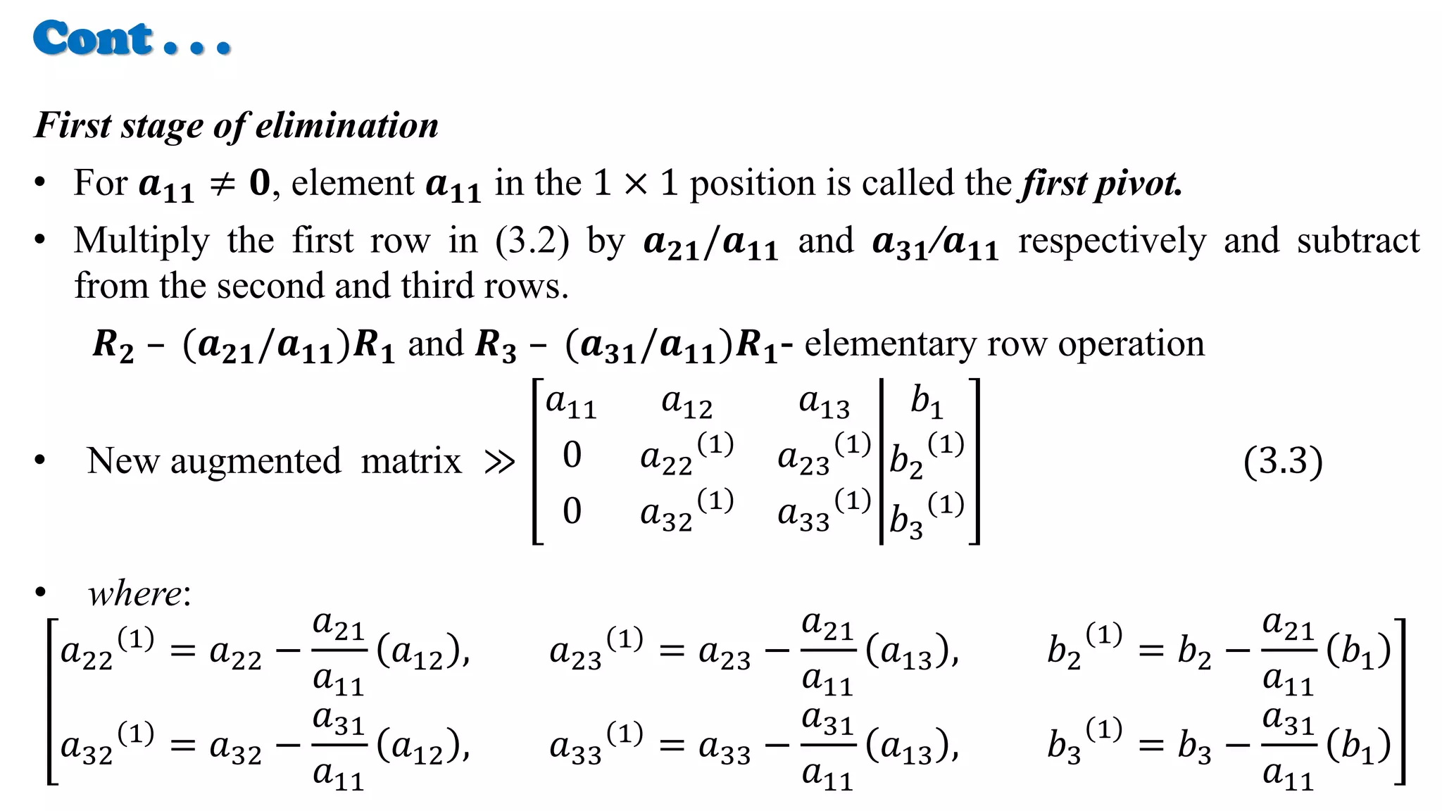
• The matrix [A | b], obtained by appending the column b to the matrix A is
called the augmented matrix. That is
𝐀 𝐛 =
𝑎11 𝑎12 … 𝑎1𝑛
𝑎21 𝑎22 … 𝑎2𝑛
. . . … … …
𝑎1𝑛 𝑎2𝑛 … 𝑎𝑛𝑛
𝑏1
𝑏2
…
𝑏𝑛](https://image.slidesharecdn.com/chapterthreeppt-210721123004/75/Numerical-Methods-3-2048.jpg)
![Cont . . .
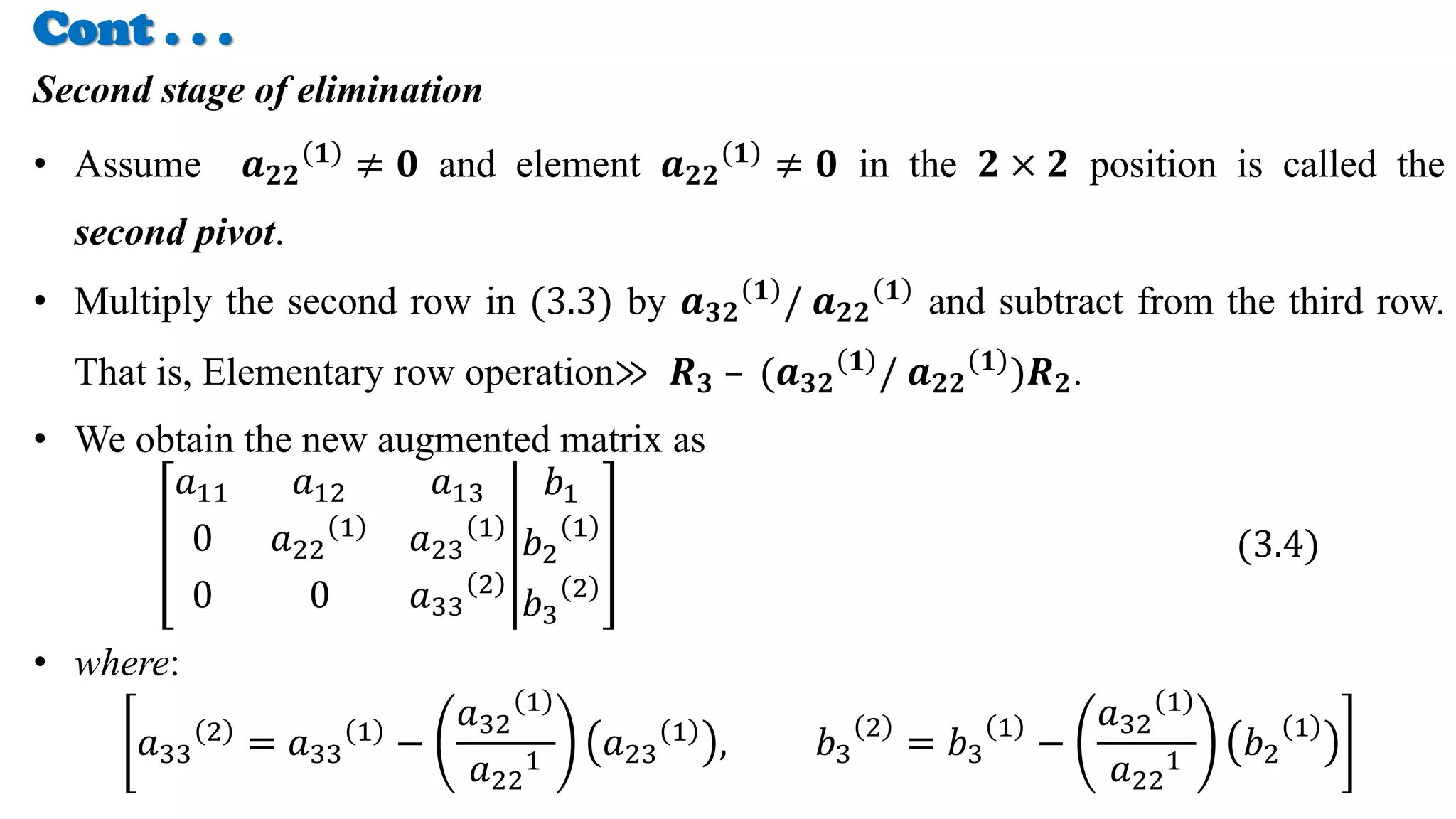
• In equation (3.4), the element 𝑎33
2
≠ 0 is called the third pivot.
• The system in (3.4), is in the required upper triangular form [𝑼|𝒛].
• The solution vector 𝒙 is now obtained by back substitution.
Back substitution:
𝒙𝟑 = 𝒃𝟑
𝟐
𝒂𝟑𝟑
𝟐
𝒙𝟐 =
𝒃𝟐
𝟏
− 𝒂𝟐𝟑
𝟏 𝒙𝟑
𝒂𝟐𝟐
𝟏
𝒙𝟏 =
(𝒃𝟏 – 𝒂𝟏𝟐𝒙𝟐 – 𝒂𝟏𝟑 𝒙𝟑)
𝒂𝟏𝟏](https://image.slidesharecdn.com/chapterthreeppt-210721123004/75/Numerical-Methods-8-2048.jpg)


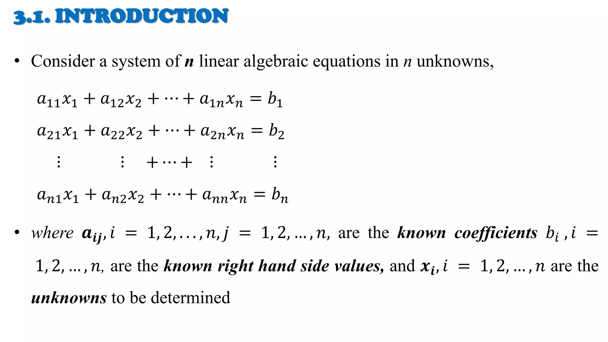
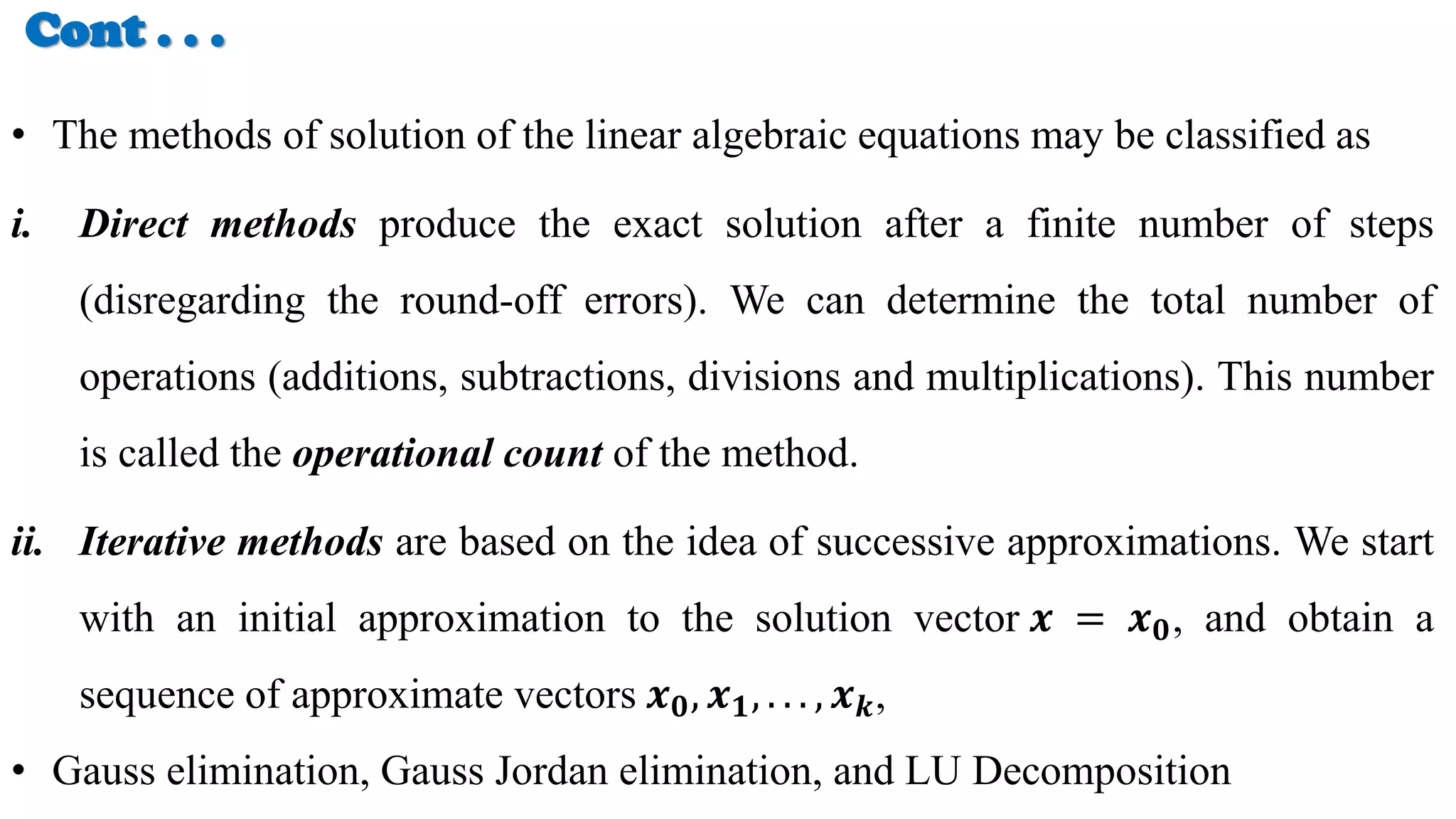
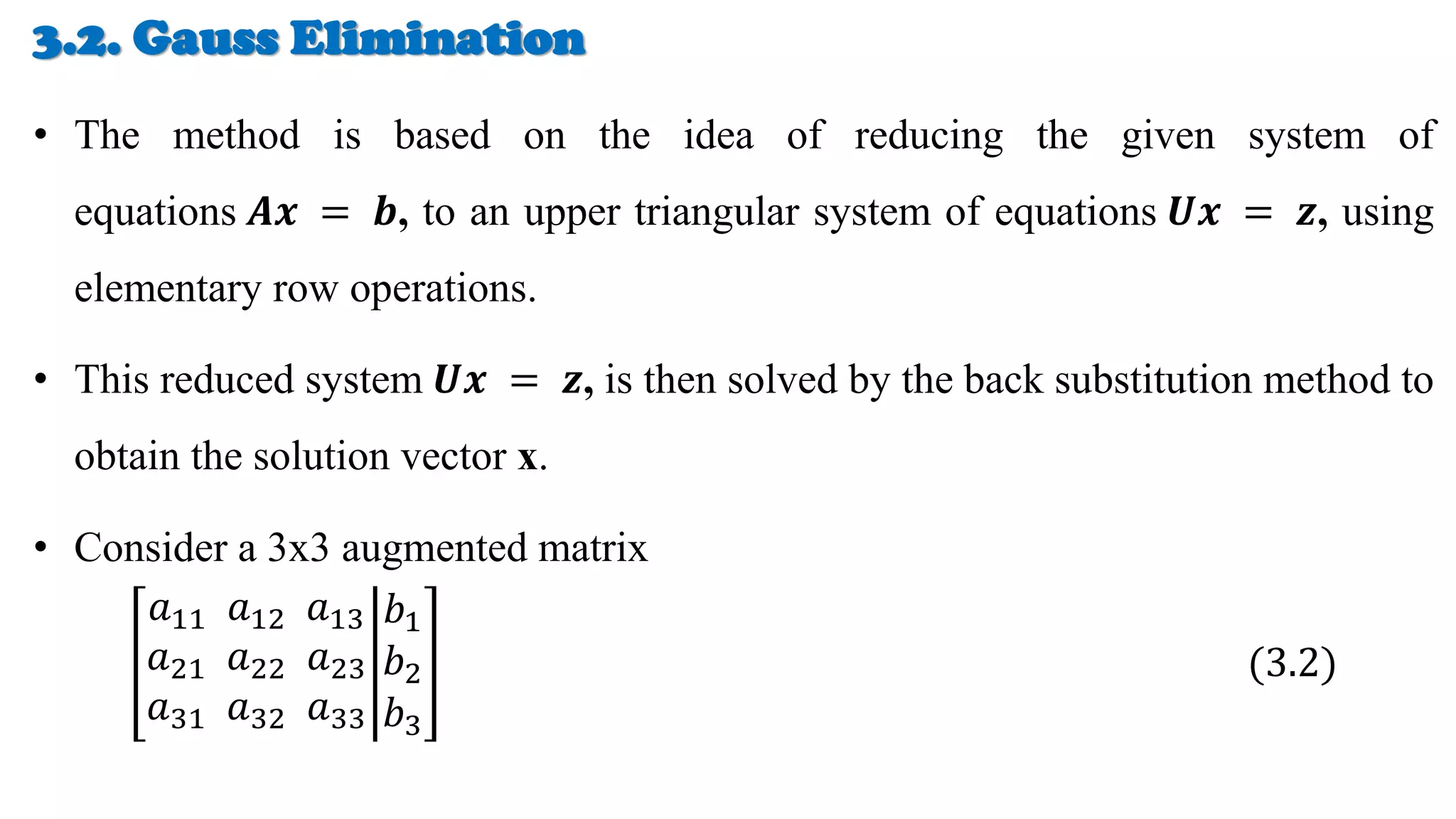
The document discusses numerical methods for solving linear algebraic equations. It begins by introducing the general form of a system of n linear equations with n unknowns. It then describes two classes of solution methods: direct and iterative. Gaussian elimination is presented as a direct method that transforms the system of equations into an upper triangular system which can then be solved using back substitution. Gauss-Seidel iteration is introduced as an iterative method that uses successive approximations to obtain solutions. The document provides examples to illustrate how to apply both Gaussian elimination and Gauss-Seidel iteration to solve systems of linear equations.
Introduction to the study of linear algebraic equations, matrix notation, and classification of solution methods. Discusses direct vs iterative methods and operational counts.
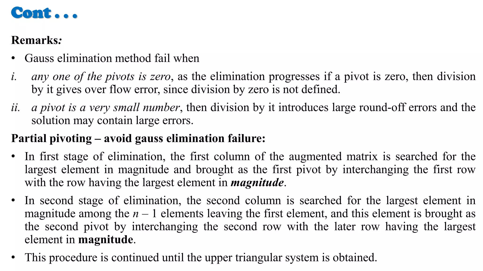
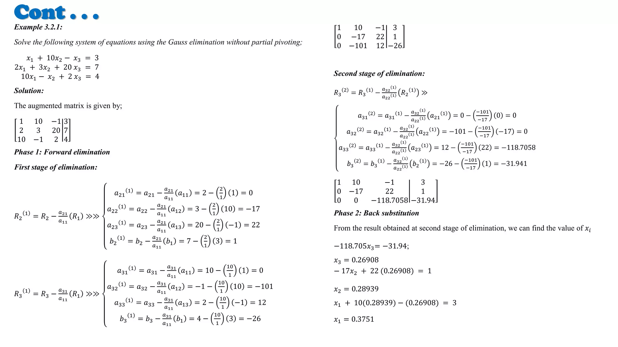
Description of the Gauss elimination approach, including stages of elimination, back substitution, and pitfalls of zero pivots. Discusses the role of partial pivoting for accuracy.
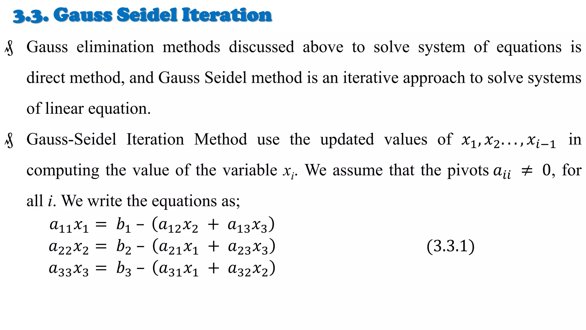
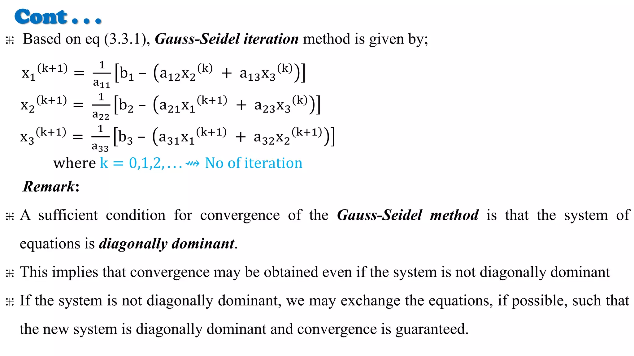
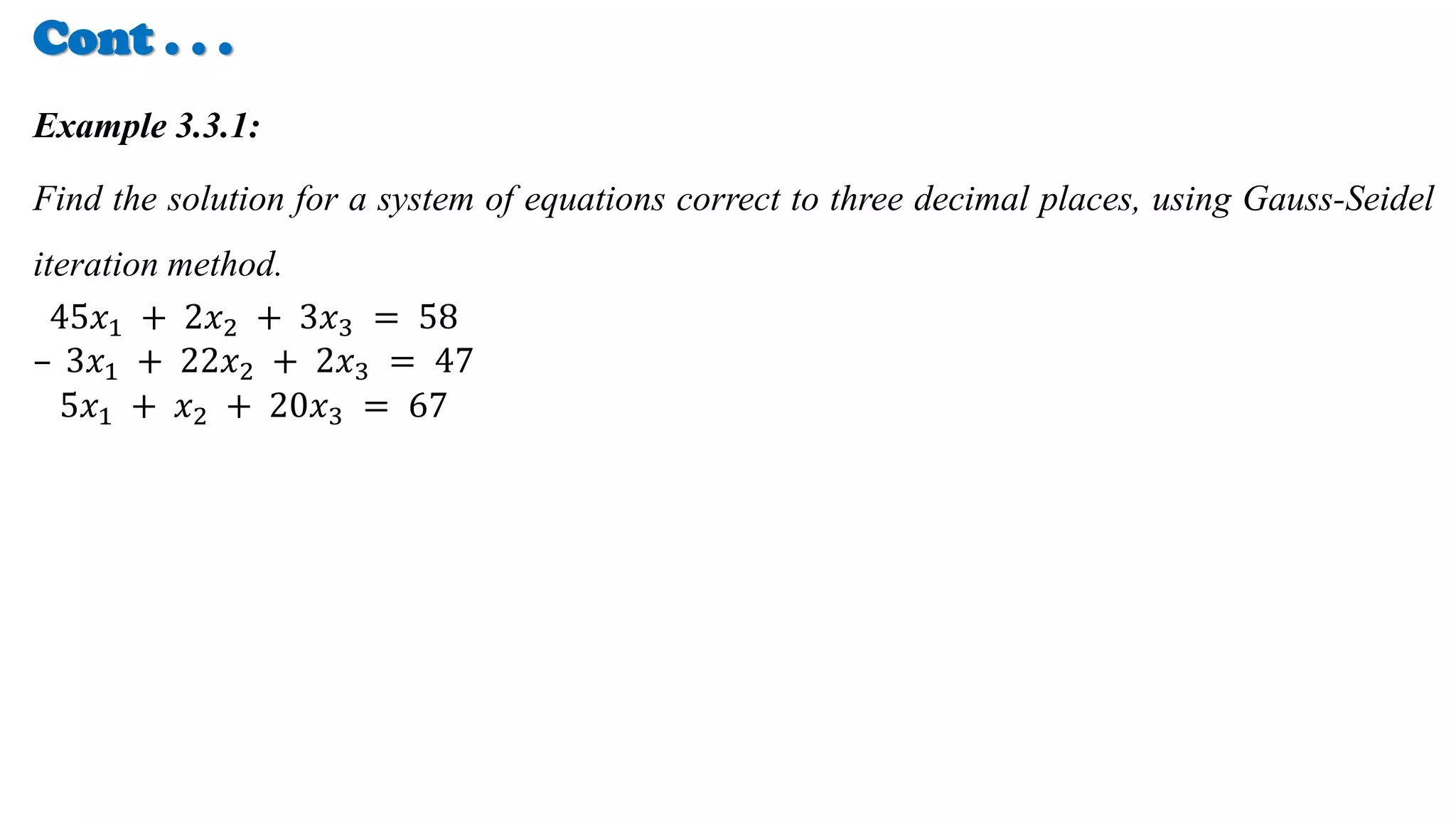
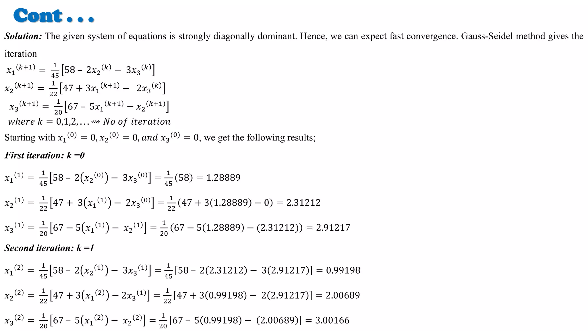
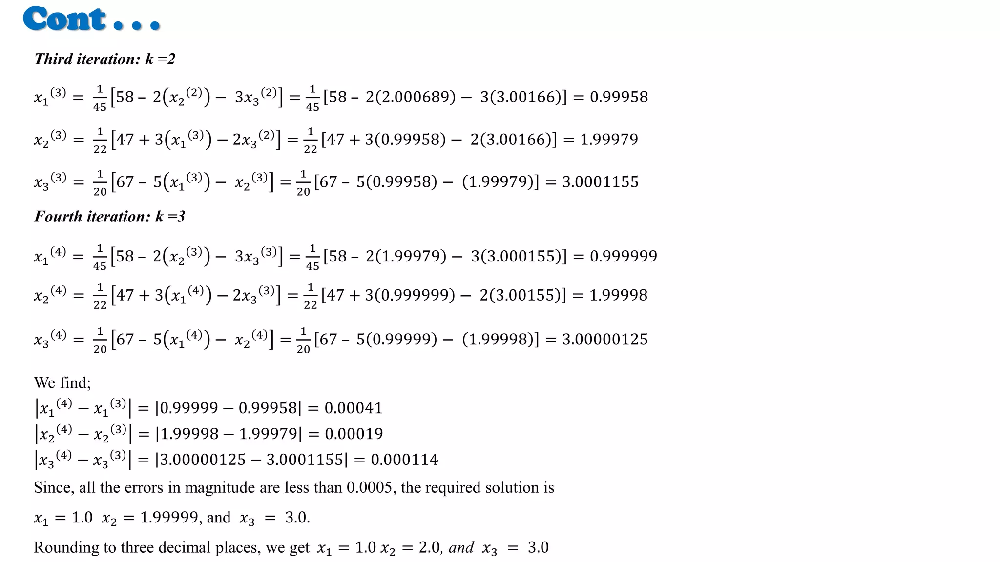
Introduction to Gauss Seidel iteration as an iterative method for solving equations, emphasizing convergence conditions and providing a detailed example with iterative solutions.
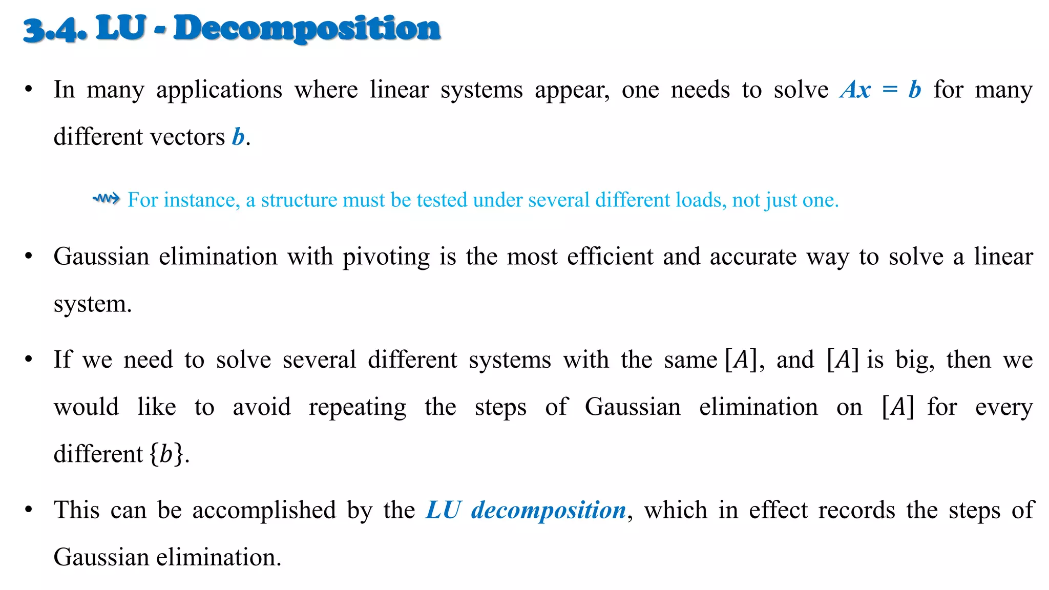
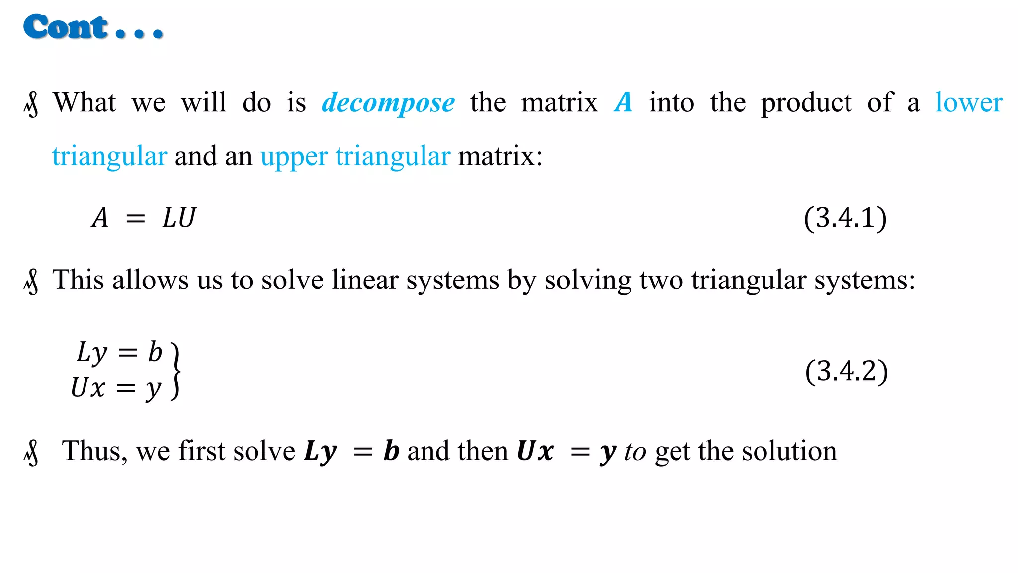
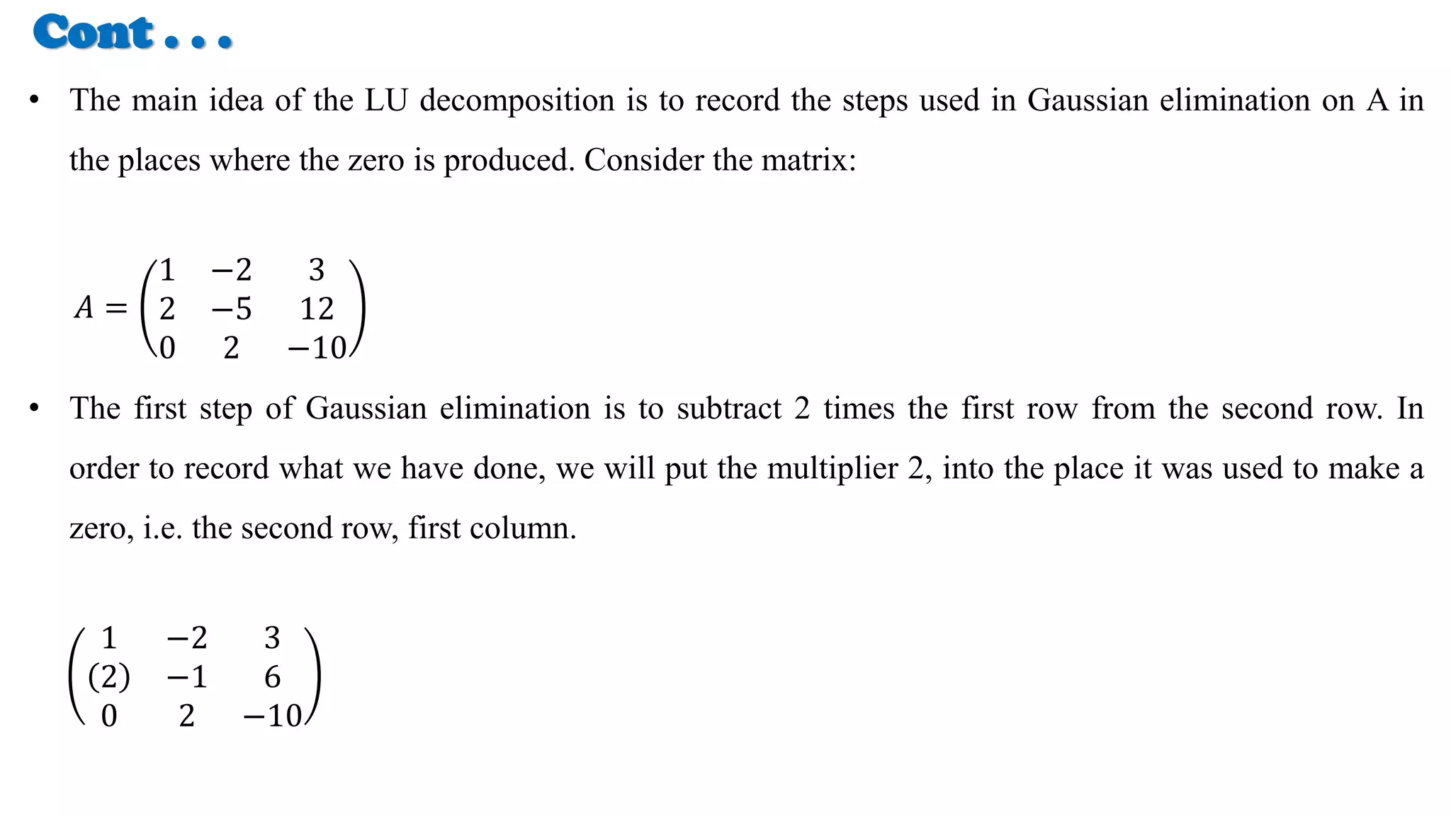
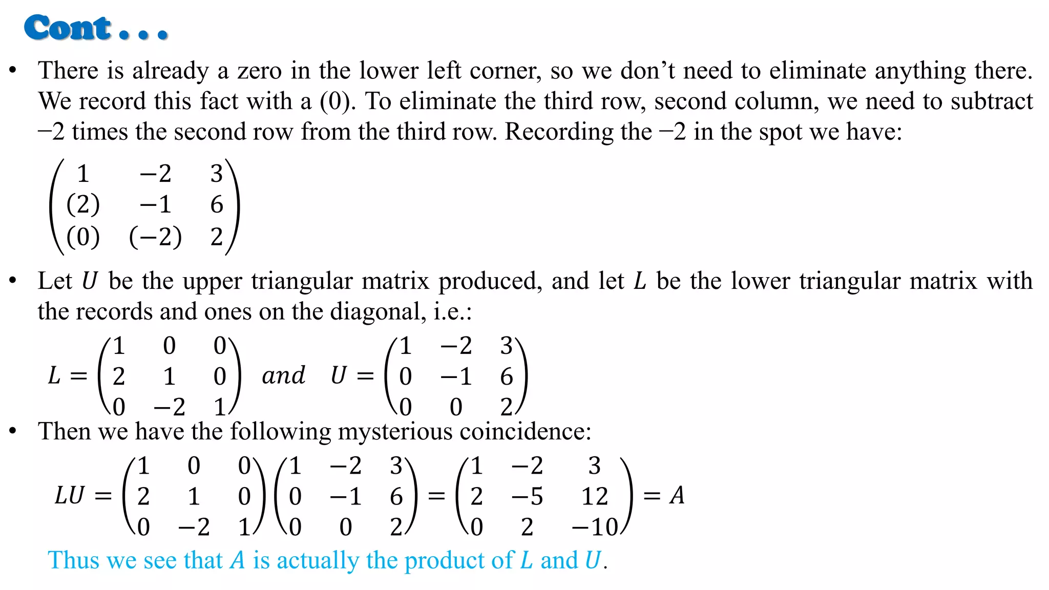
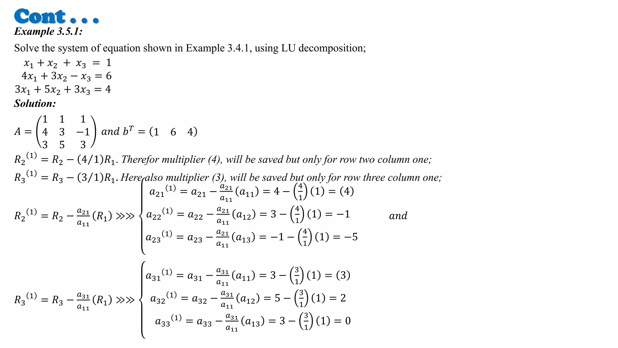
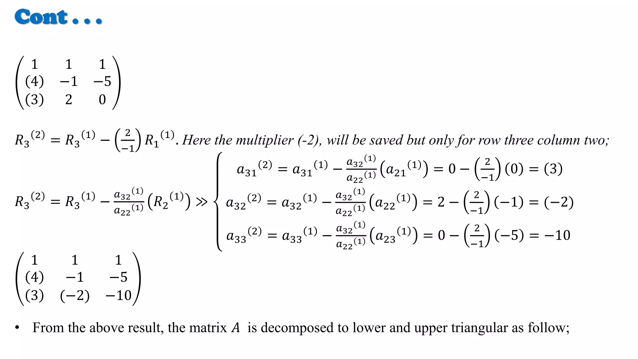
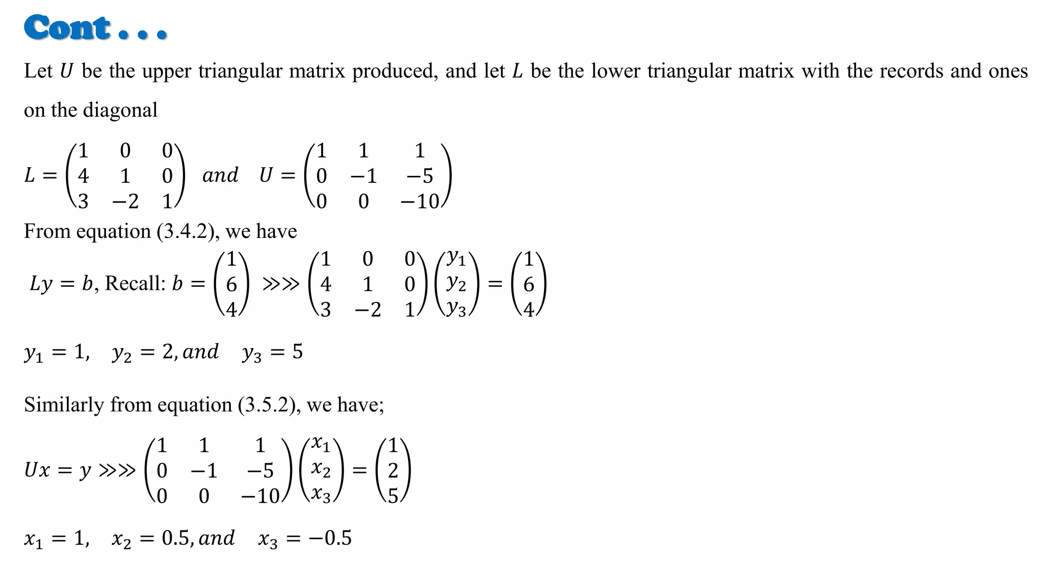
Discussion on LU decomposition for efficient resolution of linear systems, illustrating methods for matrix decomposition and providing a practical example of usage.