This document discusses matrix decomposition and its applications in statistics. It introduces several common matrix decompositions including LU, QR, Cholesky, Jordan, spectral, and singular value decompositions. The LU decomposition is described in detail, including how it can be used to solve systems of linear equations by decomposing a matrix A into lower and upper triangular matrices L and U such that A = LU. Examples are provided to demonstrate calculating the L and U matrices and using them to solve systems of linear equations.

![3
Introduction
Some of most frequently used decompositions are the LU, QR,
Cholesky, Jordan, Spectral decomposition and Singular value
decompositions.
This Lecture covers relevant matrix decompositions, basic
numerical methods, its computation and some of its applications.
Decompositions provide a numerically stable way to solve
a system of linear equations, as shown already in
[Wampler, 1970], and to invert a matrix. Additionally, they
provide an important tool for analyzing the numerical stability of
a system.](https://image.slidesharecdn.com/matrix-decomposition-and-its-application-in-statisticsnk-240418024438-7aafc94f/85/Matrix-Decomposition-and-Its-application-in-Statistics_NK-ppt-3-320.jpg)


![12
• Note: there are also generalizations of LU to non-square and singular
matrices, such as rank revealing LU factorization.
• [Pan, C.T. (2000). On the existence and computation of rank revealing LU
factorizations. Linear Algebra and its Applications, 316: 199-222.
• Miranian, L. and Gu, M. (2003). Strong rank revealing LU factorizations.
Linear Algebra and its Applications, 367: 1-16.]
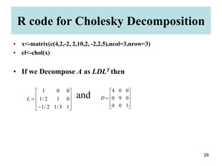
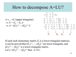
• Uses: The LU decomposition is most commonly used in the solution of
systems of simultaneous linear equations. We can also find determinant
easily by using LU decomposition (Product of the diagonal element of
upper and lower triangular matrix).
Calculation of L and U (cont.)](https://image.slidesharecdn.com/matrix-decomposition-and-its-application-in-statisticsnk-240418024438-7aafc94f/85/Matrix-Decomposition-and-Its-application-in-Statistics_NK-ppt-12-320.jpg)


![17
QR-Decomposition (Cont.)
Theorem : If A is a m×n matrix with linearly independent columns, then
A can be decomposed as , where Q is a m×n matrix whose
columns form an orthonormal basis for the column space of A and R is an
nonsingular upper triangular matrix.
Proof: Suppose A=[u1 | u2| . . . | un] and rank (A) = n.
Apply the Gram-Schmidt process to {u1, u2 , . . . ,un} and the
orthogonal vectors v1, v2 , . . . ,vn are
Let for i=1,2,. . ., n. Thus q1, q2 , . . . ,qn form a orthonormal
basis for the column space of A.
QR
A
1
2
1
1
2
2
2
2
1
2
1
1 ,
,
,
-
-
-
-
-
-
-
i
i
i
i
i
i
i
i v
v
v
u
v
v
v
u
v
v
v
u
u
v
i
i
i
v
v
q ](https://image.slidesharecdn.com/matrix-decomposition-and-its-application-in-statisticsnk-240418024438-7aafc94f/85/Matrix-Decomposition-and-Its-application-in-Statistics_NK-ppt-17-320.jpg)

![19
Let Q= [q1 q2 . . . qn] , so Q is a m×n matrix whose columns form an
orthonormal basis for the column space of A .
Now,
i.e., A=QR.
Where,
Thus A can be decomposed as A=QR , where R is an upper triangular and
nonsingular matrix.
QR-Decomposition (Cont.)
n
n
n
n
n
n
v
q
u
v
q
u
q
u
v
q
u
q
u
q
u
v
q
q
q
u
u
u
A
0
0
0
0
,
0
0
,
,
0
,
,
,
3
3
2
2
3
2
1
1
3
1
2
1
2
1
2
1
n
n
n
n
v
q
u
v
q
u
q
u
v
q
u
q
u
q
u
v
R
0
0
0
0
,
0
0
,
,
0
,
,
,
3
3
2
2
3
2
1
1
3
1
2
1
](https://image.slidesharecdn.com/matrix-decomposition-and-its-application-in-statisticsnk-240418024438-7aafc94f/85/Matrix-Decomposition-and-Its-application-in-Statistics_NK-ppt-19-320.jpg)