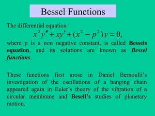
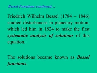
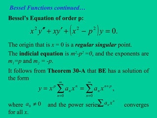
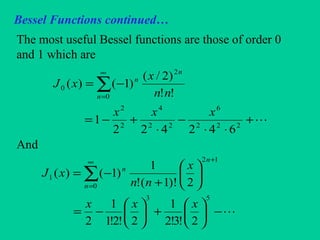
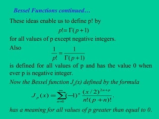
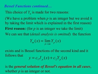
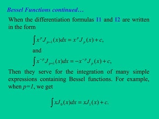
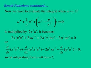
Bessel functions are solutions to Bessel's differential equation and describe oscillations that arise in many physical systems. Friedrich Bessel first systematically analyzed solutions to this equation in 1824, which became known as Bessel functions. There are Bessel functions of the first kind (Jp(x)) and second kind (Yp(x)). Jp(x) is bounded at x=0 while Yp(x) is unbounded, making them linearly independent solutions for the general solution. The gamma function was developed to define Bessel functions for all real values of p.


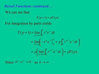
![Bessel Functions continued…
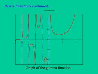
Properties of Bessel Functions:
The Bessel function Jp(x) is defined for any real number
p by
Identities and the function Jm+1/2(x).
We prove the following identity
∑
∞
=
+
+
−=
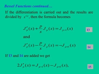
0
2
.
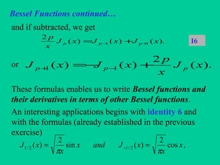
)!(!
)2/(
)1()(
n
pn
n
p
npn
x
xJ
[ ] )()( 1 xJxxJx
dx
d
p
p
p
p
−= I1](https://image.slidesharecdn.com/3besselsfunctions-181005210418/85/3-bessel-s-functions-29-320.jpg)
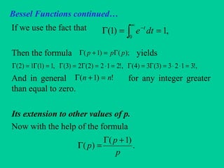
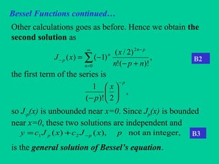
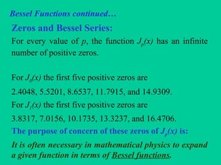
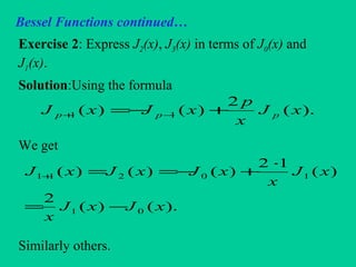
![Bessel Functions continued…
Proof:
[ ]
)(
)!1(!
)2/()1(
)!1(!2
)1(
)!(!2
)1(
)(
1
0
12
0
12
122
0
2
22
xJx
npn
x
x
npn
x
npn
x
dx
d
xJx
dx
d
p
p
n
pnn
p
n
pn
pnn
n
pn
pnn
p
p
−
∞
=
−+
∞
=
−+
−+
∞
=
+
+
=
−+
−
=
−+
−
=
+
−
=
∑
∑
∑](https://image.slidesharecdn.com/3besselsfunctions-181005210418/85/3-bessel-s-functions-30-320.jpg)
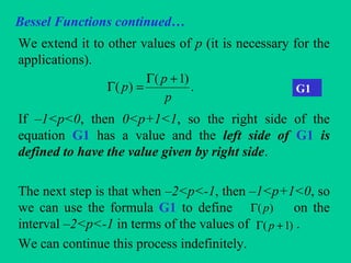
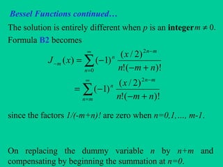
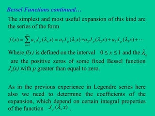
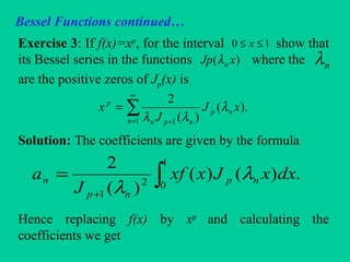
![Bessel Functions continued…
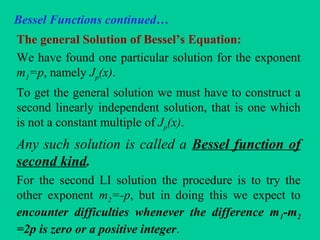
And the second identity is
Proof:
[ ] ).()( 1 xJxxJx
dx
d
p
p
p
p
+
−−
−= I2
[ ]
).(
)!1(!
)2/()1(
)!()!1(2
)1(
)!(!2
)1(
)(
1
0
12
1
12
12
0
2
2
xJx
npn
x
x
npn
x
npn
x
dx
d
xJx
dx
d
p
p
n
pnn
p
n
pn
nn
n
pn
nn
p
p
+
−
∞
=
++
−
∞
=
−+
−
∞
=
+
−
−=
++
−
−=
+−
−
=
+
−
=
∑
∑
∑](https://image.slidesharecdn.com/3besselsfunctions-181005210418/85/3-bessel-s-functions-31-320.jpg)
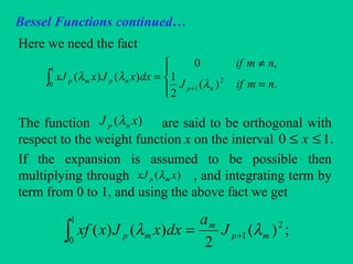
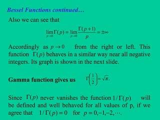
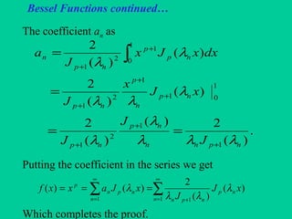
![Bessel Functions continued…
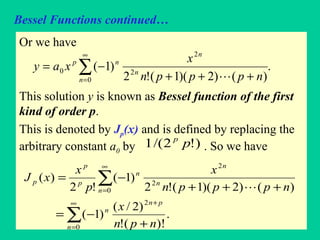
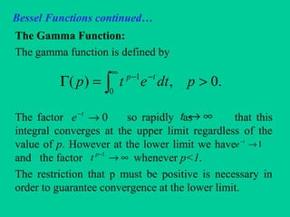
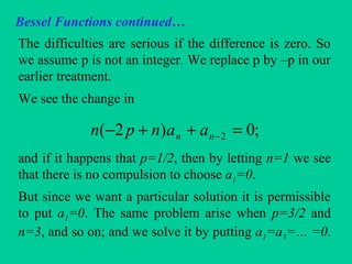
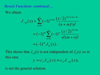
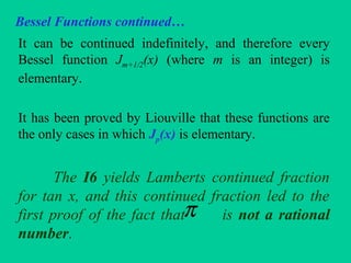
This theorem is given without proof which tells about
the conditions under which the series actually converges.
Theorem A. (Bessel expansion theorem).
Assume that f(x) and have at most finite
number of jump discontinuities on the interval
. If 0<x<1, then the Bessel series
converges to f(x) when x is a point of continuity
of this function, and converges to
when x is a point of discontinuity.
)(xf ′
10 ≤≤ x
[ ])()(
2
1
++− xfxf](https://image.slidesharecdn.com/3besselsfunctions-181005210418/85/3-bessel-s-functions-41-320.jpg)

( 1
0
1
0
22
uvvuxdxxuvab ′−′=− ∫
∫ =
1
0
,0)()( dxxJxxJ npmp λλ
mλ nλ
).()()()( aubvbvau ′−′](https://image.slidesharecdn.com/3besselsfunctions-181005210418/85/3-bessel-s-functions-46-320.jpg)
![Bessel Functions continued…
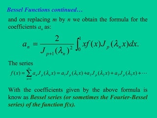
we obtain
when x=0. The expression in brackets vanishes; and
since we get
Now putting we get
since Jp(a)=0 and
and the proof of the second part is complete.
,])([2 1
0
222222
1
0
22
upxauxdxxua −+′=∫
),()1( aJau p
′=′
.)(1
2
1
)(
2
1
)( 2
2
2
2
1
0
2
aJ
a
p
aJdxaxxJ ppp
−+′=∫
na λ=
,)(
2
1
)(
2
1
)( 2
1
2
1
0
2
npnpnp JJdxxxJ λλλ +=′=∫
)()()()()( 11 npnpppp JJxJxJ
x
p
xJ λλ ++ =
′
⇒=−
′](https://image.slidesharecdn.com/3besselsfunctions-181005210418/85/3-bessel-s-functions-48-320.jpg)
;()( 0110 xxJxxJ
dx
d
xJxJ
dx
d
=−=
[ ]
).(
)!1(!
)2/()1(
)!1(!
)2/()1(
!!2
2)1(
!!2
)1(
)(
1
0
121
1
12
1
2
12
0
2
2
0
xJ
nn
x
nn
x
nn
nx
nn
x
dx
d
xJ
dx
d
n
nn
n
nn
n
n
nn
n
n
nn
−=
+
−
=
−
−
=
−
=
−
=
∑∑
∑∑
∞
=
++∞
=
−
∞
=
−∞
=](https://image.slidesharecdn.com/3besselsfunctions-181005210418/85/3-bessel-s-functions-49-320.jpg)
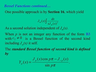
![Bessel Functions continued…
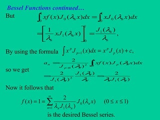
Suppose x1 and x2 are any two positive zeros of J0(x), then
J0(x1)=0=J0(x2) and J0(x) is differentiable for all positive
values of x.
But by Rolle’s theorem if f(x) is continuous on [a,b] and
differentiable on (a,b) and f(a)=f(b)=0 then there exists at
least one number c in (a,b) such that
Hence applying this theorem there exists at least one
number x3 in (x1, x2) such that
Hence in between any two positive zeros of J0(x) there is
a zero for J1(x). Other part is left to you.
.0)( =′ cf
.0)(.0)()(or0)( 31313030 ==−=
′
=
′
xJeixJxJxJ](https://image.slidesharecdn.com/3besselsfunctions-181005210418/85/3-bessel-s-functions-50-320.jpg)
![Bessel Functions continued…
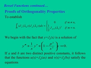
Exercise 4: Prove that
Solution:
[ ] [ ].)()()()(
2
1
2
1 xJxJxxJxxJ
dx
d
pppp ++ −=
[ ] [ ]
[ ] [ ]
[ ]
[ ].)()(
)()()()(
)()()()(
)()()()(
2
1
2
11
11
1
1
1
1
1
1
1
xJxJx
xJxxJxxJxxJx
xJx
dx
d
xJxxJx
dx
d
xJx
xJxxJx
dx
d
xJxxJ
dx
d
pp
p
p
p
p
p
p
p
p
p
p
p
p
p
p
p
p
p
p
p
p
pp
+
+
−
+
++−
−
+
+
+
+−
+
+−
+
−=
−+=
+=
=](https://image.slidesharecdn.com/3besselsfunctions-181005210418/85/3-bessel-s-functions-54-320.jpg)