Download as PDF, PPTX
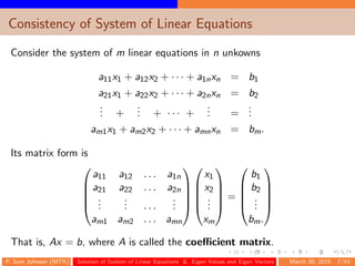
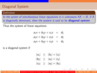
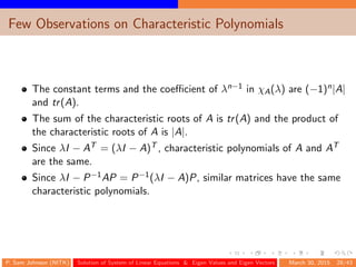
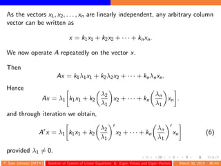
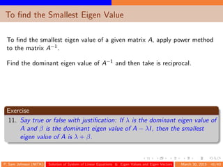
![To determine whether these equations are consistent or not, we find the
ranks of the coefficient matrix A and the augmented matrix
K =
a11 a12 . . . a1n b1
a21 a22 . . . a2n b2
...
... · · ·
...
...
am1 am2 . . . amn bm
= [A b].
We denote the rank of A by r(A).
1. r(A) = r(K), then the linear system Ax = b is inconsistent and has
no solution.
2. r(A) = r(K) = n, then the linear system Ax = b is consistent and
has a unique solution.
3. r(A) = r(K) < n, then the linear system Ax = b is consistent and
has an infinite number of solutions.
P. Sam Johnson (NITK) Solution of System of Linear Equations & Eigen Values and Eigen Vectors March 30, 2015 8/43](https://image.slidesharecdn.com/solutiontolinearequations-150416123121-conversion-gate02/85/Solution-to-linear-equhgations-8-320.jpg)
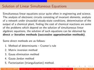
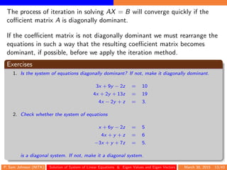
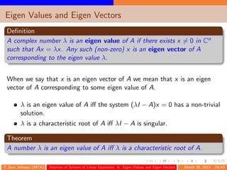
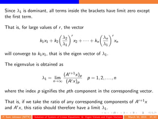
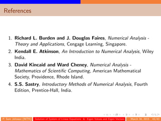
![Rayeigh’s Power Method
Similarly, we evaluate Ax(2) = λ(2)x(2) which gives the second
approximation. We repeat this process till [x(r) − x(r−1)] becomes
negligible.
Then λ(r) will be the dominant (largest) eigen value and x(r), the
corresponding eigen vector (dominant eigen vector).
The iteration method of finding the dominant eigen value of a square
matrix is called the Rayeigh’s power method.
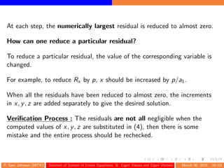
At each stage of iteration, we take out the largest component from y(r) to
find x(r) where
y(r+1)
= Ax(r)
, r = 0, 1, 2, . . . .
P. Sam Johnson (NITK) Solution of System of Linear Equations & Eigen Values and Eigen Vectors March 30, 2015 40/43](https://image.slidesharecdn.com/solutiontolinearequations-150416123121-conversion-gate02/85/Solution-to-linear-equhgations-40-320.jpg)
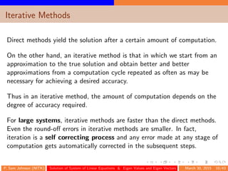
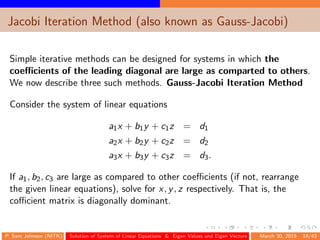
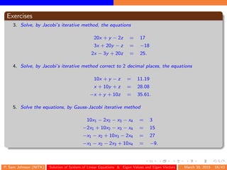
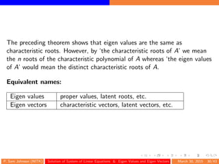
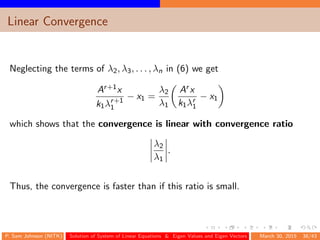
![Exercises
12. Determine the largest eigen value and the corresponding eigen vector
of the matrix
5 4
1 2
.
13. Find the largest eigen value and the corresponding eigen vector of the
matrix
2 −1 0
−1 2 −1
0 −1 2
using power method. Take [1, 0, 0]T as an initial eigen vector.
14. Obtain by power method, the numerically dominant eigen value and
eigen vector of the matrix
15 −4 −3
−10 12 −6
−20 4 −2.
P. Sam Johnson (NITK) Solution of System of Linear Equations & Eigen Values and Eigen Vectors March 30, 2015 42/43](https://image.slidesharecdn.com/solutiontolinearequations-150416123121-conversion-gate02/85/Solution-to-linear-equhgations-42-320.jpg)

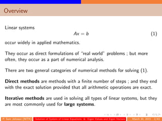
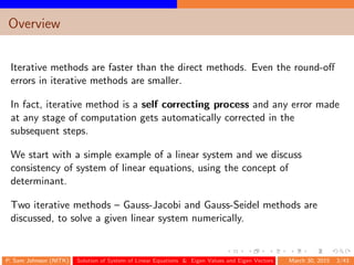
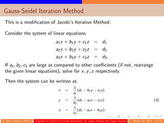
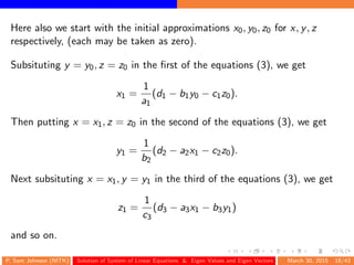
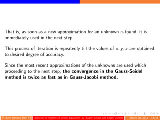
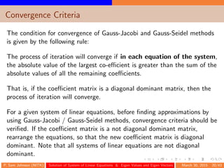
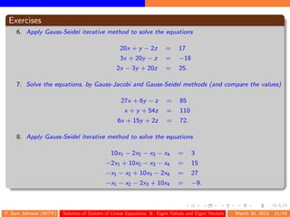
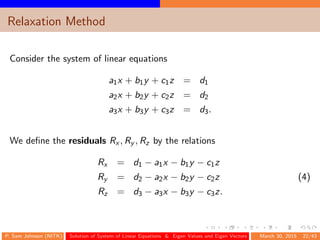
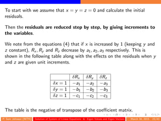
1. The document discusses methods for solving systems of linear equations and calculating eigen values and eigen vectors of matrices. It describes direct and iterative methods for solving linear systems, including Gauss-Jacobi and Gauss-Seidel iterative methods. 2. It also covers the concepts of diagonal dominance and consistency conditions for linear systems. Rayleigh's power method is introduced for finding the dominant eigen value and vector of a matrix. 3. Examples are provided to illustrate solving linear systems by Jacobi's method and checking for diagonal dominance and consistency of systems. The convergence criteria for Gauss-Jacobi and Gauss-Seidel methods are also outlined.