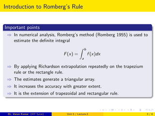
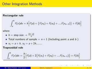
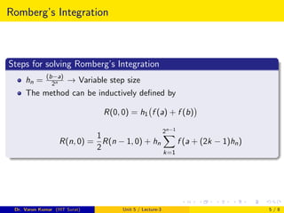
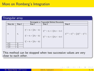
Romberg’s Integration
Dr. Varun Kumar
Dr. Varun Kumar (IIIT Surat) Unit 5 / Lecture-3 1 / 8
Outlines
1 Introduction to Romberg’s Rule
2 Mathematical Formulation
3 Example
Dr. Varun Kumar (IIIT Surat) Unit 5 / Lecture-3 2 / 8
Introduction to Romberg’s Rule
Important points
⇒ In numerical analysis, Romberg’s method (Romberg 1955) is used to
estimate the definite integral
F(x) =
Z b
a
f (x)dx
⇒ By applying Richardson extrapolation repeatedly on the trapezium
rule or the rectangle rule.
⇒ The estimates generate a triangular array.
⇒ It increases the accuracy with greater extent.
⇒ It is the extension of trapezoidal and rectangular rule.
Dr. Varun Kumar (IIIT Surat) Unit 5 / Lecture-3 3 / 8
Other Integration Methods
Rectangular rule
Z b
a
f (x)dx = h
h
f (a) +

f (x1) + f (x2) + ....f (xn−1)
	
+ f (b)
i
where
h = step size → (b−a)
n
Total numbers of sample = n + 1 (Including point a and b )
x1 = a + h, x2 = a + 2h,.......
Trapezoidal rule
Z b
a
f (x)dx =
h
2
h
f (a) + 2

f (x1) + f (x2) + ....f (xn−1)
	
+ f (b)
i
Dr. Varun Kumar (IIIT Surat) Unit 5 / Lecture-3 4 / 8
Romberg’s Integration
Steps for solving Romberg’s Integration
hn = (b−a)
2n → Variable step size
The method can be inductively defined by
R(0, 0) = h1 f (a) + f (b)

R(n, 0) =
1
2
R(n − 1, 0) + hn
2n−1
X
k=1
f (a + (2k − 1)hn)
Dr. Varun Kumar (IIIT Surat) Unit 5 / Lecture-3 5 / 8
More on Romberg’s Integration
Triangular array
Rectangular or Trapezoidal Method Recursively
Step size Step-1 Step-2 Step-3 Step-4
h I1
I∗
1 = I2 + 1
3
(I2 − I1)
I∗
2 = I3 + 1
3
(I3 − I2)
I∗
3 = I4 + 1
3
(I4 − I3)
I∗∗
1 = I2 ∗ + 1
3
(I2 ∗ −I1∗)
I∗∗
2 = I3 ∗ + 1
3
(I3 ∗ −I2∗)
I∗∗∗
1 = I∗∗
1 + 1
3
(I∗∗
2 − I∗∗
1 )
h/2 I2
h/4 I3
h/8 I4
This method can be stopped when two successive values are very
close to each other.
Dr. Varun Kumar (IIIT Surat) Unit 5 / Lecture-3 6 / 8
Example–
Example
Q Evaluate the following definite integral J using Romberg’s integration
rule, where
J =
Z 1
0
1
1 + x
dx
Ans Solution: According to question, a = 0, b = 1. We solve this by
trapezoidal rule
Case 1: Taking h = 0.5, the value of x and f (x) is
At x = 0, f (x) = 1
At x = 0.5, f (x) = 0.66667
At x = 1, f (x) = 0.5
At I = 1
4[1 + 2 × 0.66667 + 0.5] = 0.70835
Dr. Varun Kumar (IIIT Surat) Unit 5 / Lecture-3 7 / 8
Continued–
Case 2: Taking h = 0.25, the value of x and f (x) is
x 0 0.25 0.5 0.75 1
f(x) 1 0.8 0.667 0.5714 0.5
By trapezoidal rule I = 0.25
2 [1 + 2(0.8 + 0.667 + 0.5714) + 0.5] = 0.6970
Case 3: Taking h=0.125, x and f (x) value is
x 0 0.125 0.25 0.375 0.5 0.625 0.75 0.875 1
f(x) 1 0.8889 0.8 0.7273 0.667 0.6154 0.5714 0.5333 0.5
By trapezoidal rule
I = 0.125
2
[1+2(0.8889+0.8+0.7273+0.667+0.6154+0.5714+0.5333)+0.5] = 0.6914
I(h) = 0.7084 I(h/2) = 0.6970 I(h/4) = 0.6914
I∗
1 = 0.6932, I∗
2 = 0.6931 and I∗∗
1 = 0.6931
Dr. Varun Kumar (IIIT Surat) Unit 5 / Lecture-3 8 / 8

Romberg's Integration

  • 1.
    Romberg’s Integration Dr. VarunKumar Dr. Varun Kumar (IIIT Surat) Unit 5 / Lecture-3 1 / 8
  • 2.
    Outlines 1 Introduction toRomberg’s Rule 2 Mathematical Formulation 3 Example Dr. Varun Kumar (IIIT Surat) Unit 5 / Lecture-3 2 / 8
  • 3.
    Introduction to Romberg’sRule Important points ⇒ In numerical analysis, Romberg’s method (Romberg 1955) is used to estimate the definite integral F(x) = Z b a f (x)dx ⇒ By applying Richardson extrapolation repeatedly on the trapezium rule or the rectangle rule. ⇒ The estimates generate a triangular array. ⇒ It increases the accuracy with greater extent. ⇒ It is the extension of trapezoidal and rectangular rule. Dr. Varun Kumar (IIIT Surat) Unit 5 / Lecture-3 3 / 8
  • 4.
    Other Integration Methods Rectangularrule Z b a f (x)dx = h h f (a) + f (x1) + f (x2) + ....f (xn−1) + f (b) i where h = step size → (b−a) n Total numbers of sample = n + 1 (Including point a and b ) x1 = a + h, x2 = a + 2h,....... Trapezoidal rule Z b a f (x)dx = h 2 h f (a) + 2 f (x1) + f (x2) + ....f (xn−1) + f (b) i Dr. Varun Kumar (IIIT Surat) Unit 5 / Lecture-3 4 / 8
  • 5.
    Romberg’s Integration Steps forsolving Romberg’s Integration hn = (b−a) 2n → Variable step size The method can be inductively defined by R(0, 0) = h1 f (a) + f (b) R(n, 0) = 1 2 R(n − 1, 0) + hn 2n−1 X k=1 f (a + (2k − 1)hn) Dr. Varun Kumar (IIIT Surat) Unit 5 / Lecture-3 5 / 8
  • 6.
    More on Romberg’sIntegration Triangular array Rectangular or Trapezoidal Method Recursively Step size Step-1 Step-2 Step-3 Step-4 h I1 I∗ 1 = I2 + 1 3 (I2 − I1) I∗ 2 = I3 + 1 3 (I3 − I2) I∗ 3 = I4 + 1 3 (I4 − I3) I∗∗ 1 = I2 ∗ + 1 3 (I2 ∗ −I1∗) I∗∗ 2 = I3 ∗ + 1 3 (I3 ∗ −I2∗) I∗∗∗ 1 = I∗∗ 1 + 1 3 (I∗∗ 2 − I∗∗ 1 ) h/2 I2 h/4 I3 h/8 I4 This method can be stopped when two successive values are very close to each other. Dr. Varun Kumar (IIIT Surat) Unit 5 / Lecture-3 6 / 8
  • 7.
    Example– Example Q Evaluate thefollowing definite integral J using Romberg’s integration rule, where J = Z 1 0 1 1 + x dx Ans Solution: According to question, a = 0, b = 1. We solve this by trapezoidal rule Case 1: Taking h = 0.5, the value of x and f (x) is At x = 0, f (x) = 1 At x = 0.5, f (x) = 0.66667 At x = 1, f (x) = 0.5 At I = 1 4[1 + 2 × 0.66667 + 0.5] = 0.70835 Dr. Varun Kumar (IIIT Surat) Unit 5 / Lecture-3 7 / 8
  • 8.
    Continued– Case 2: Takingh = 0.25, the value of x and f (x) is x 0 0.25 0.5 0.75 1 f(x) 1 0.8 0.667 0.5714 0.5 By trapezoidal rule I = 0.25 2 [1 + 2(0.8 + 0.667 + 0.5714) + 0.5] = 0.6970 Case 3: Taking h=0.125, x and f (x) value is x 0 0.125 0.25 0.375 0.5 0.625 0.75 0.875 1 f(x) 1 0.8889 0.8 0.7273 0.667 0.6154 0.5714 0.5333 0.5 By trapezoidal rule I = 0.125 2 [1+2(0.8889+0.8+0.7273+0.667+0.6154+0.5714+0.5333)+0.5] = 0.6914 I(h) = 0.7084 I(h/2) = 0.6970 I(h/4) = 0.6914 I∗ 1 = 0.6932, I∗ 2 = 0.6931 and I∗∗ 1 = 0.6931 Dr. Varun Kumar (IIIT Surat) Unit 5 / Lecture-3 8 / 8