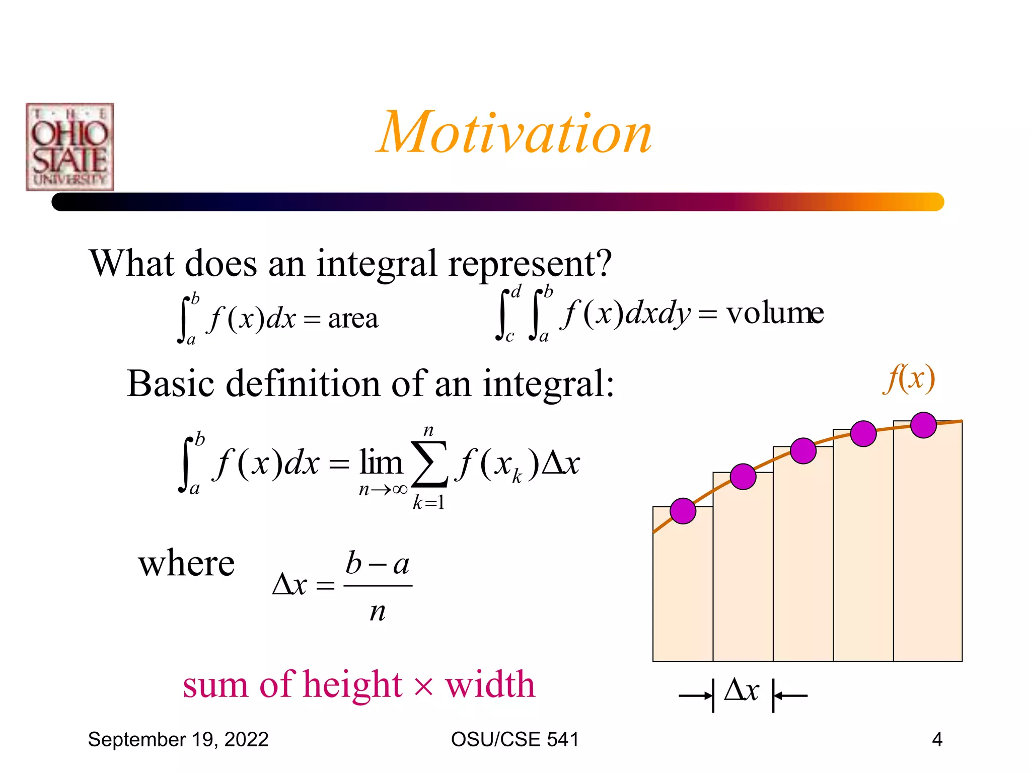
This document discusses numerical integration techniques. It begins by defining definite integrals and introducing the concepts of lower and upper Riemann sums. It then describes various quadrature rules for approximating integrals, including the trapezoid rule, Simpson's rule, Gaussian quadrature, and adaptive Simpson's method. It explains how these rules replace the integral with a weighted sum using different polynomial approximations within intervals of the bounded region. The document provides examples applying the trapezoid rule and estimating associated errors.
![September 19, 2022 OSU/CSE 541 7
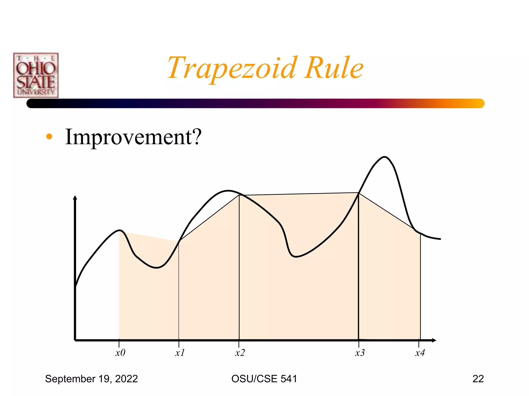
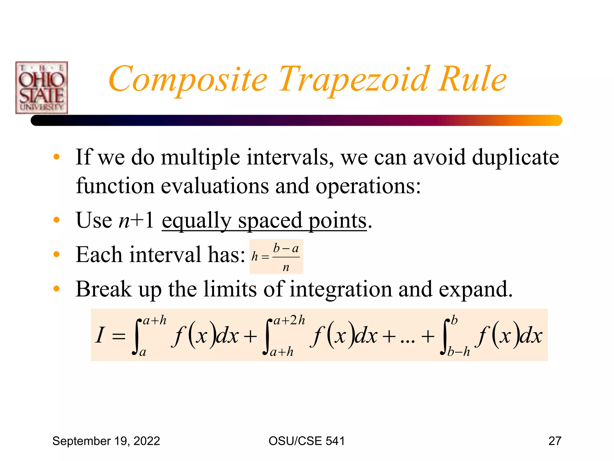
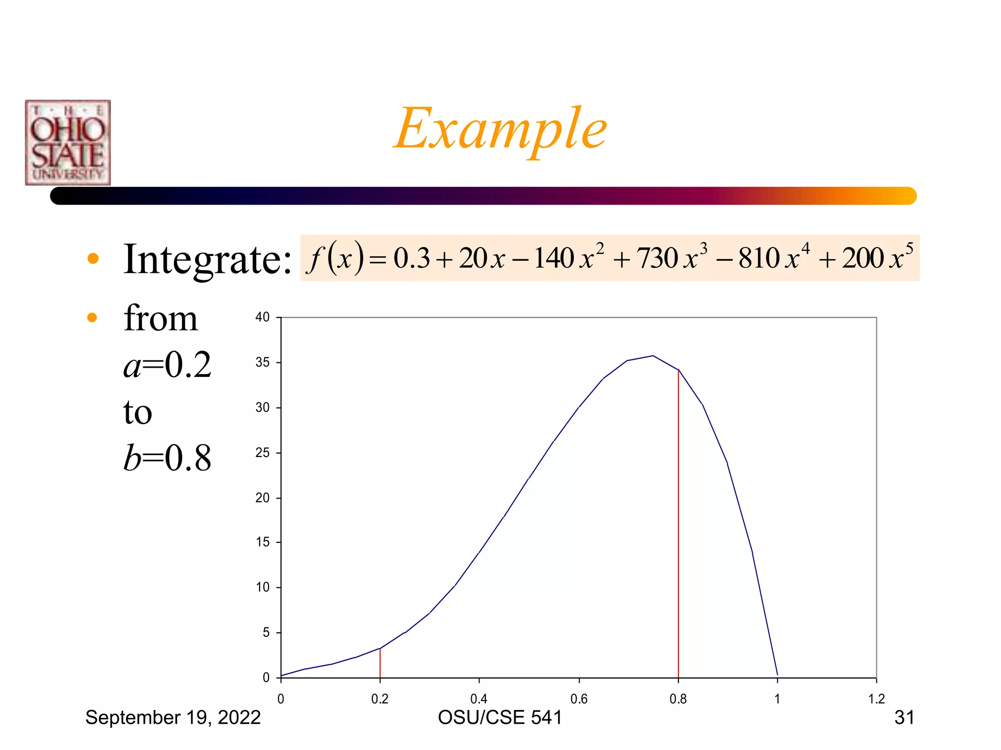
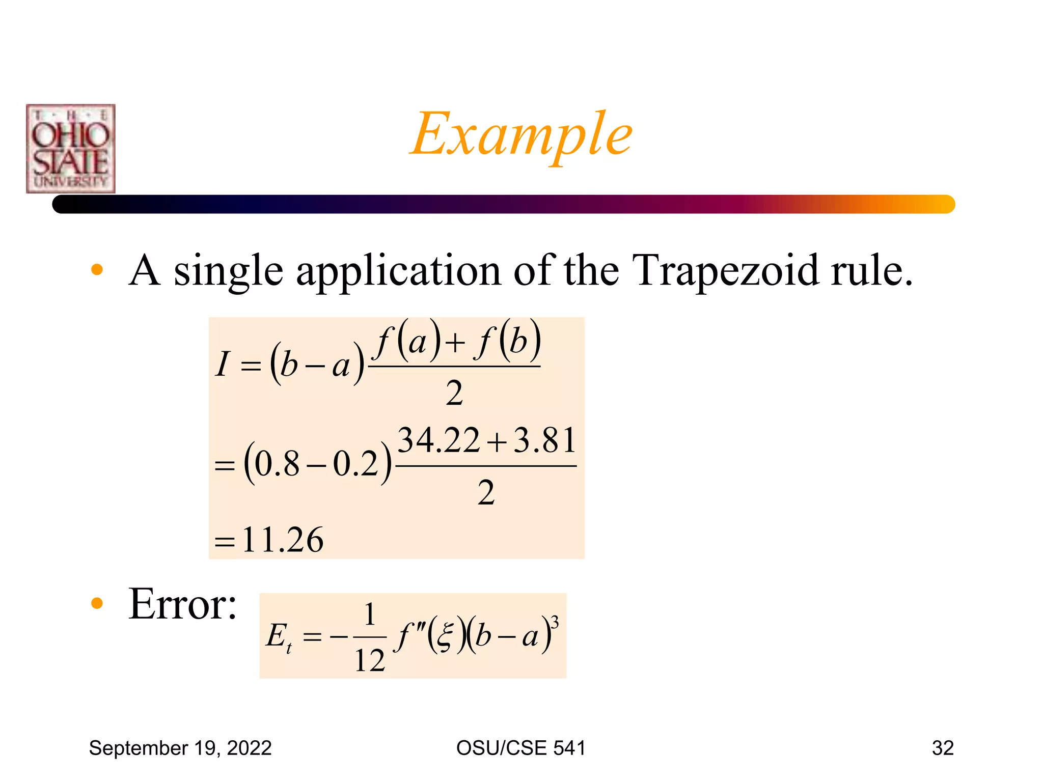
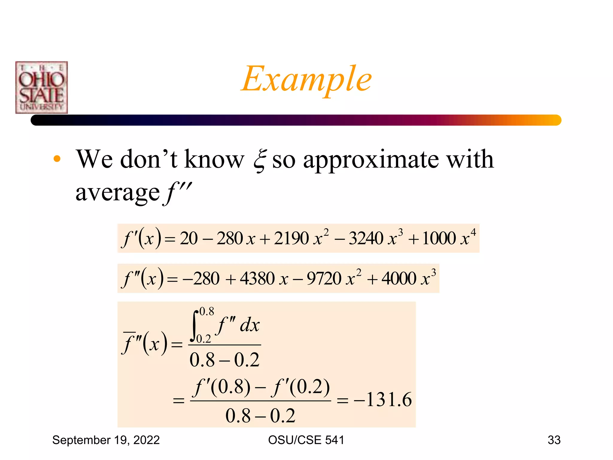
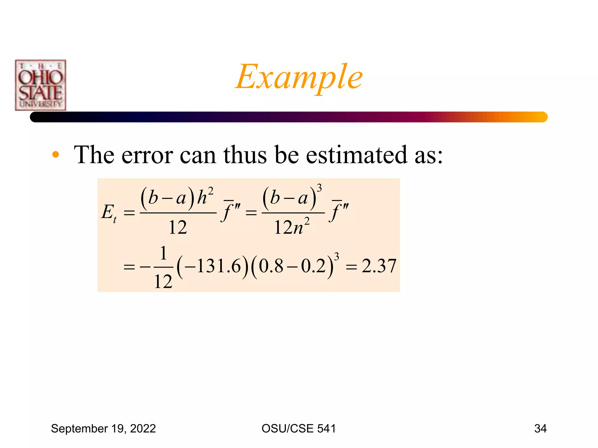
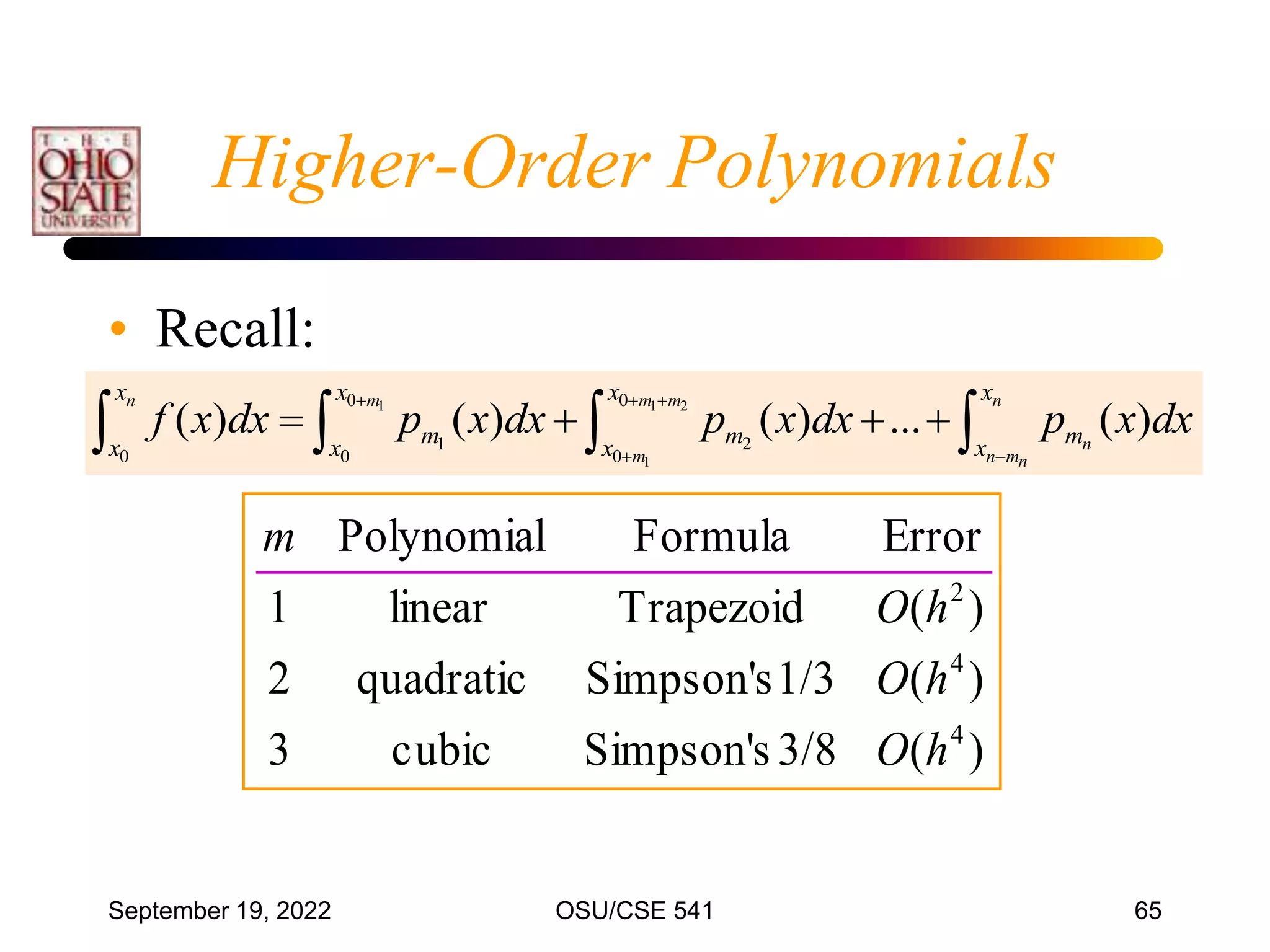
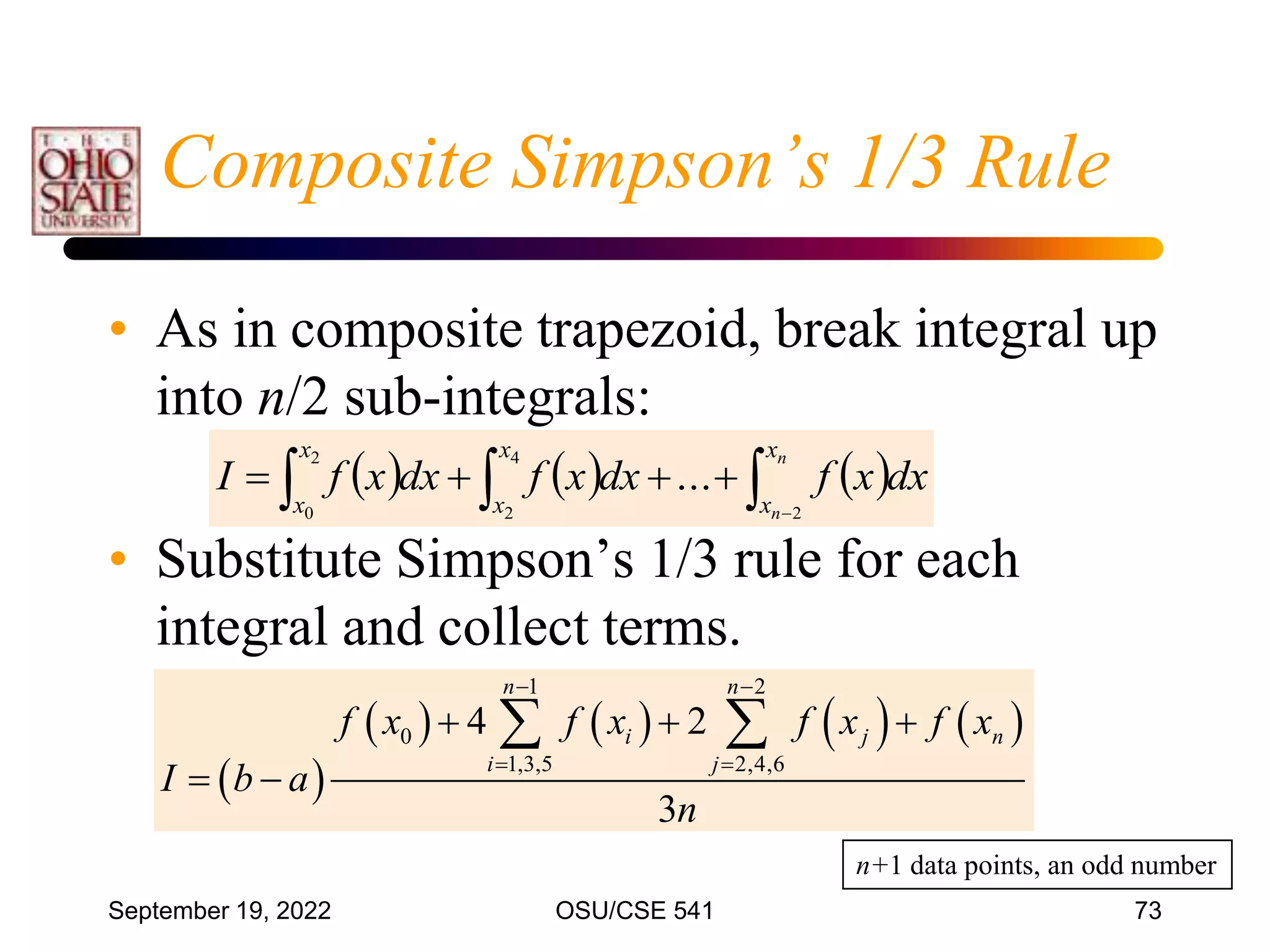
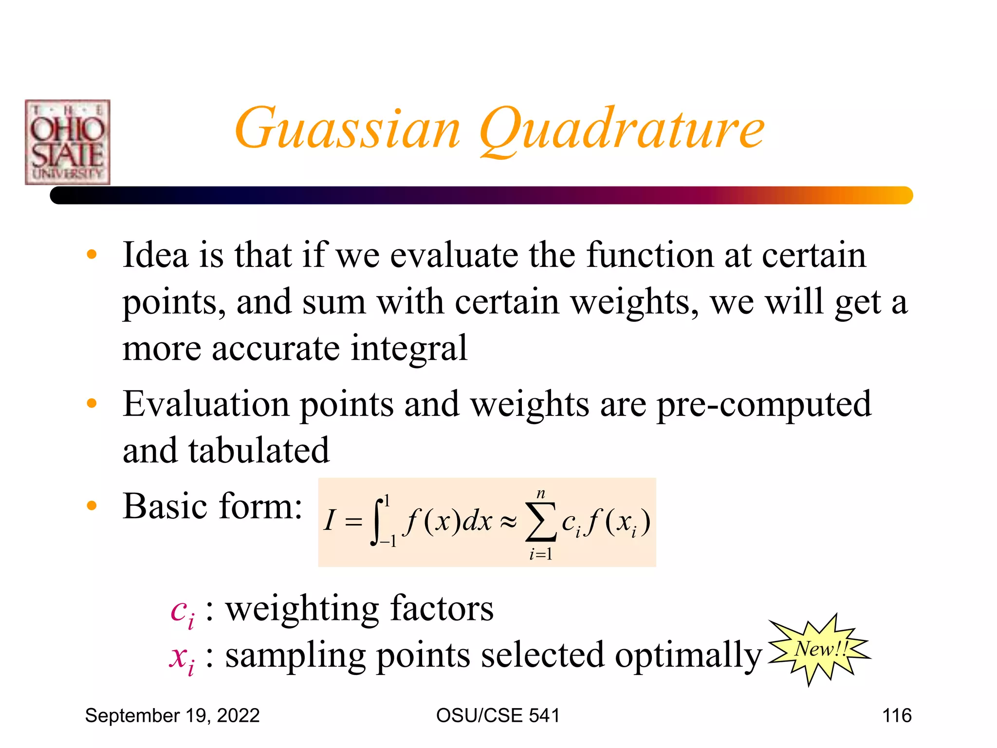
• The most common numerical integration formula
is based on equally spaced data points.
• Divide [x0 , xn] into n intervals (n1)
n
x
x
dx
x
f
0
)
(
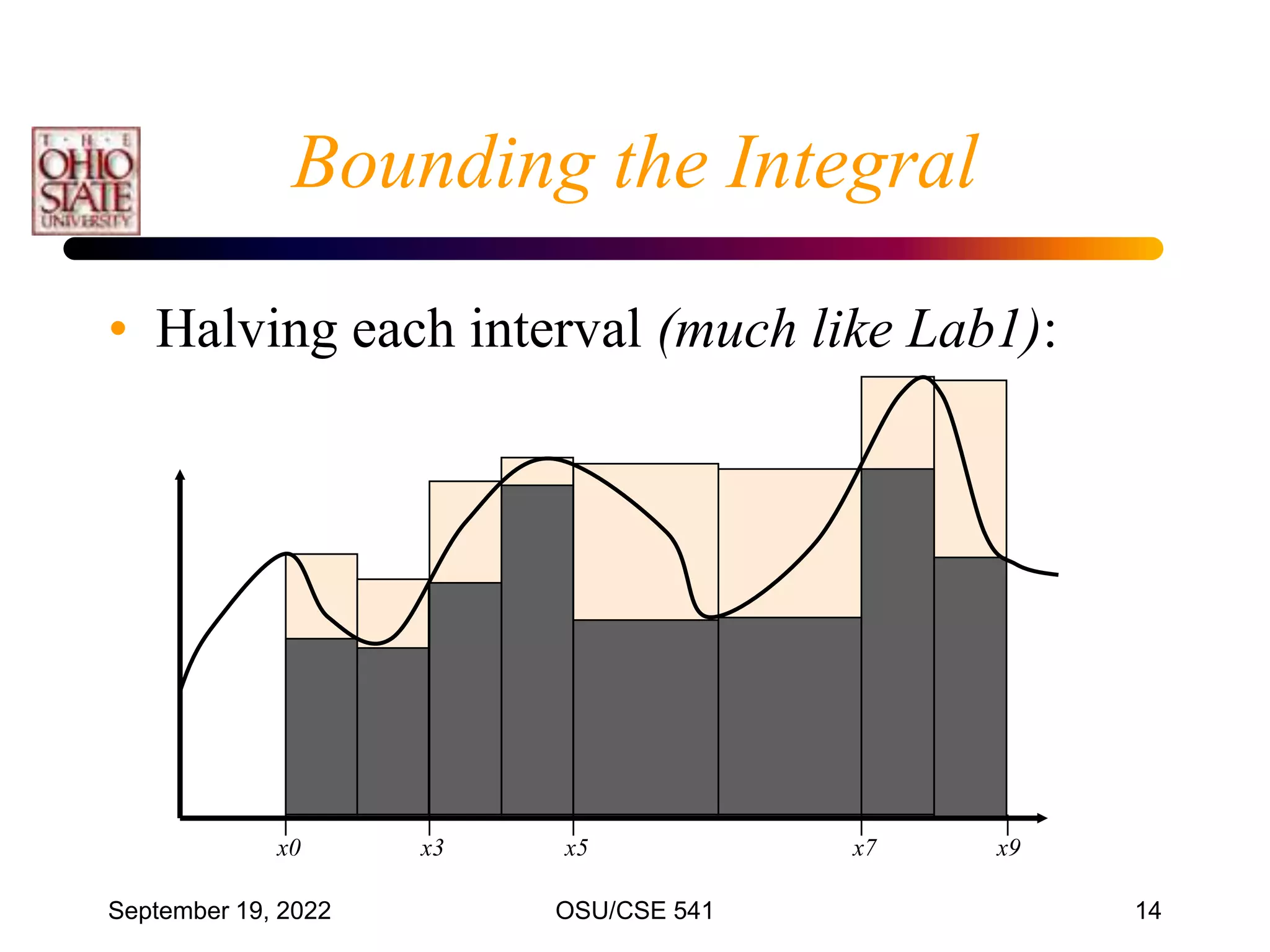
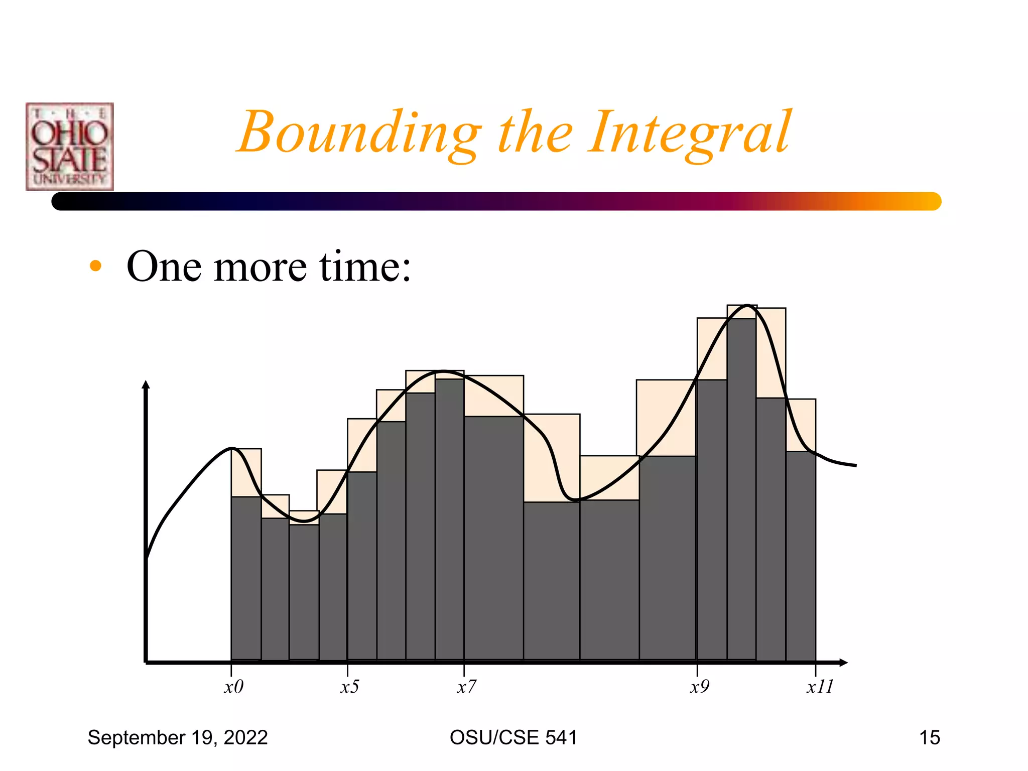
Partitioning the Integral
1 2
0
0 1 1
( ) ( ) ( ) ( )
n
n
n
x
x x
x
x
x x x
f x dx f x f x f x
](https://image.slidesharecdn.com/cis54107integration-220919040837-b4ac4cde/75/CIS541_07_Integration-ppt-7-2048.jpg)
![September 19, 2022 OSU/CSE 541 26
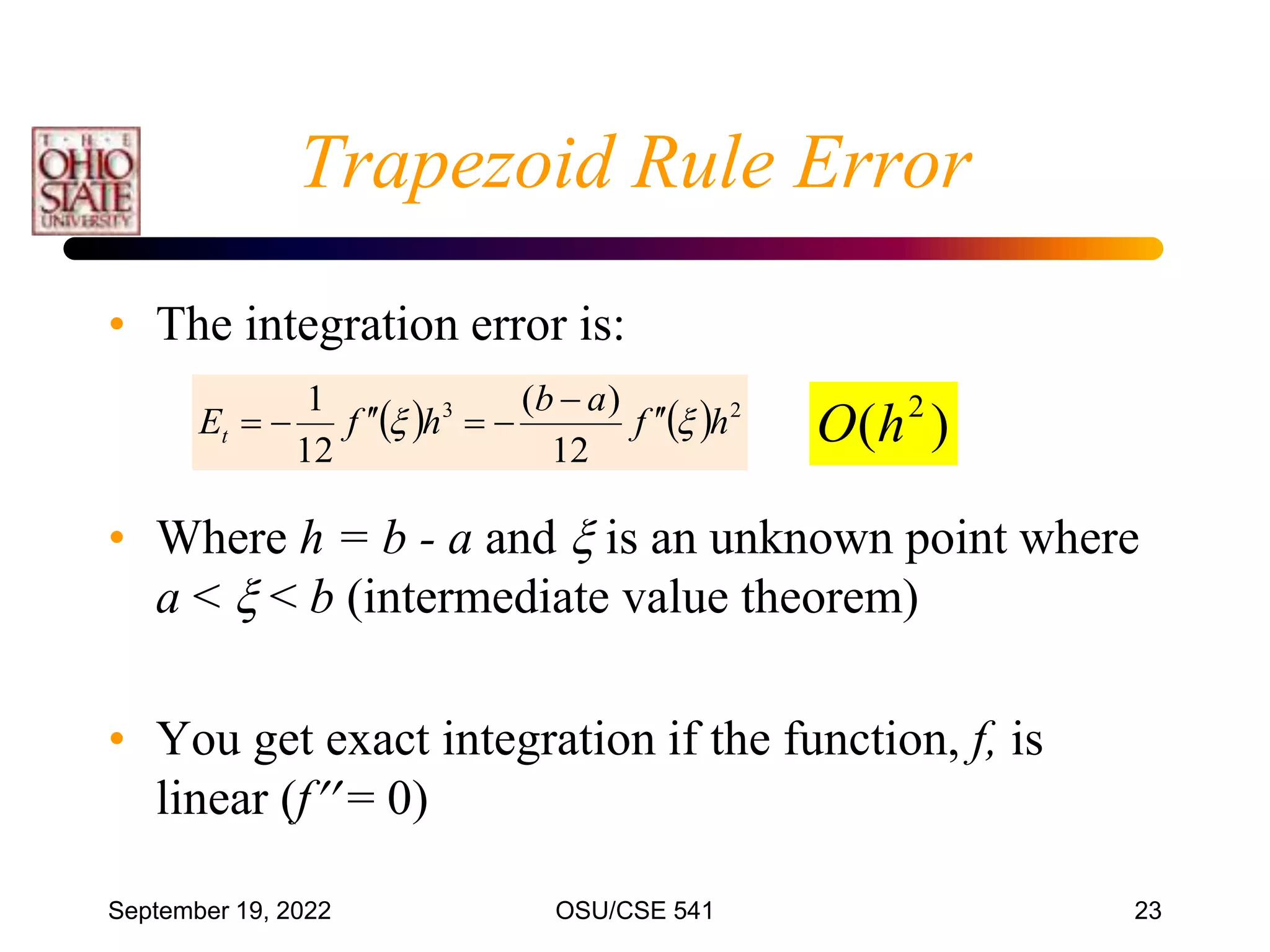
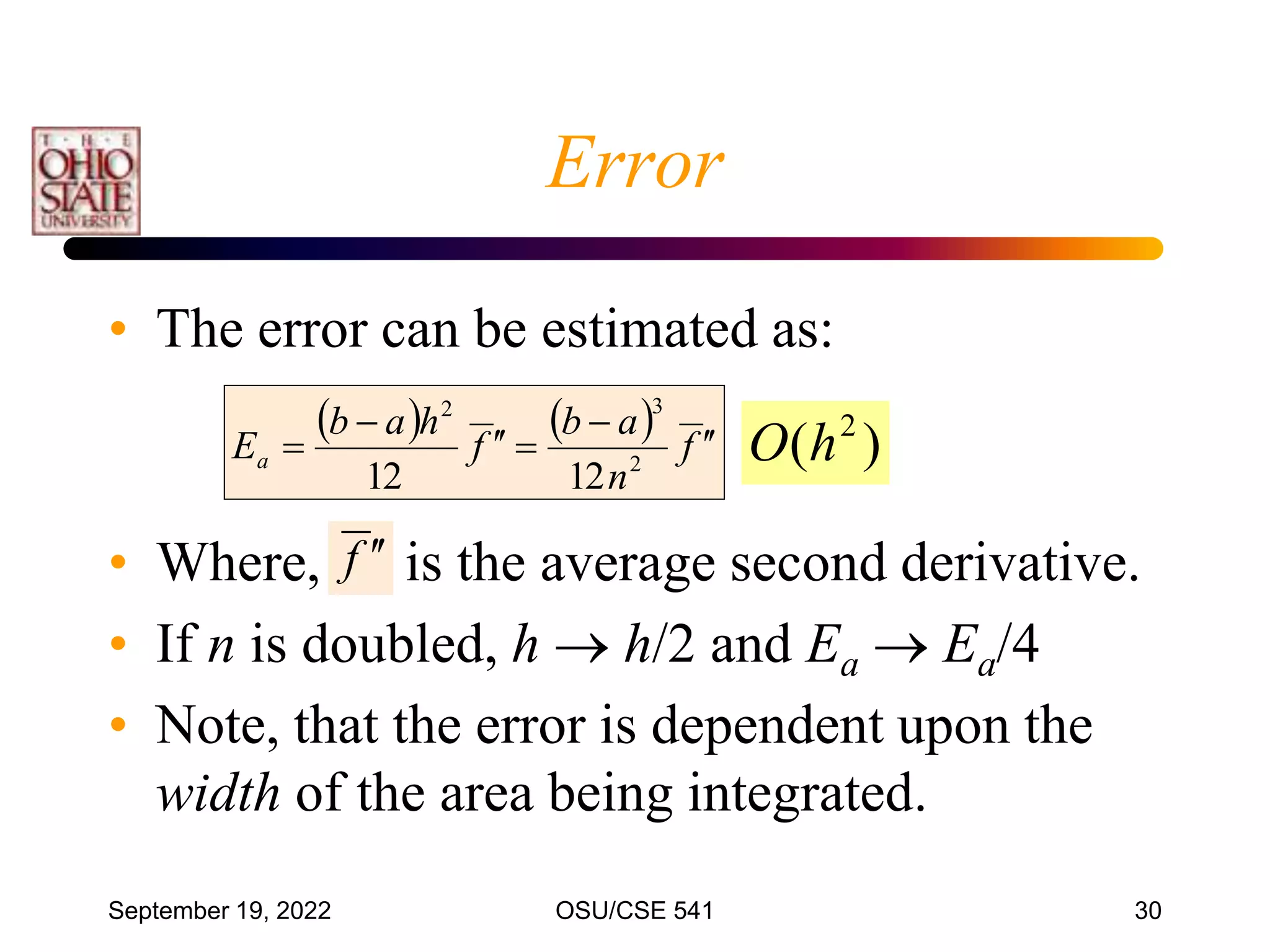
More intervals, better result [error O(h2)]
0
1
2
3
4
5
6
7
3 5 7 9 11 13 15
n = 2
0
1
2
3
4
5
6
7
3 5 7 9 11 13 15
n = 3
0
1
2
3
4
5
6
7
3 5 7 9 11 13 15
n = 4
0
1
2
3
4
5
6
7
3 5 7 9 11 13 15
n = 8](https://image.slidesharecdn.com/cis54107integration-220919040837-b4ac4cde/75/CIS541_07_Integration-ppt-26-2048.jpg)
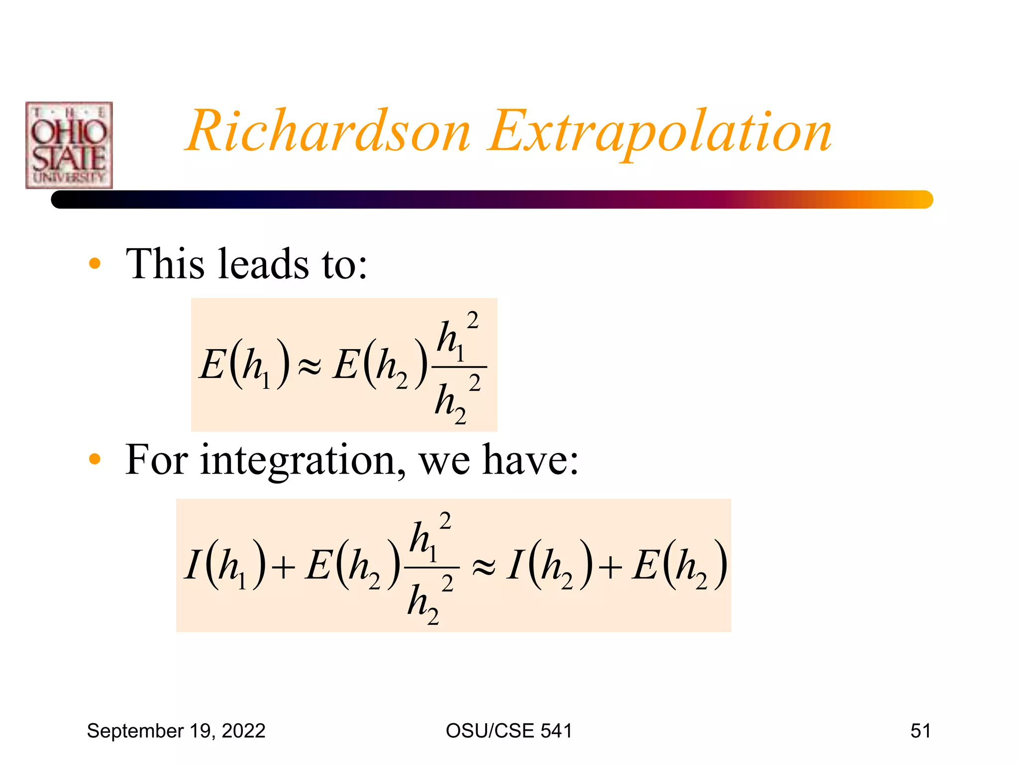
![September 19, 2022 OSU/CSE 541 50
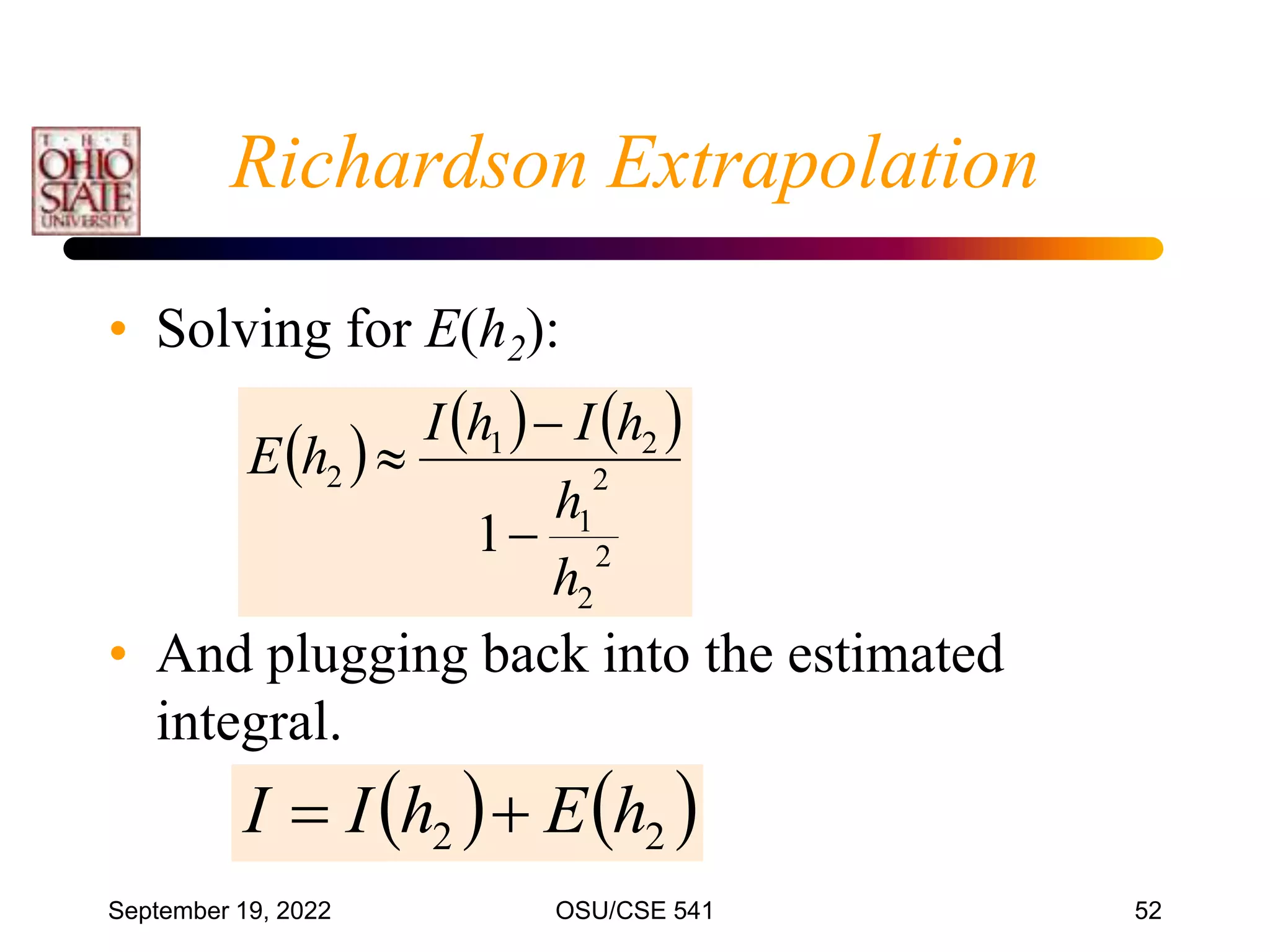
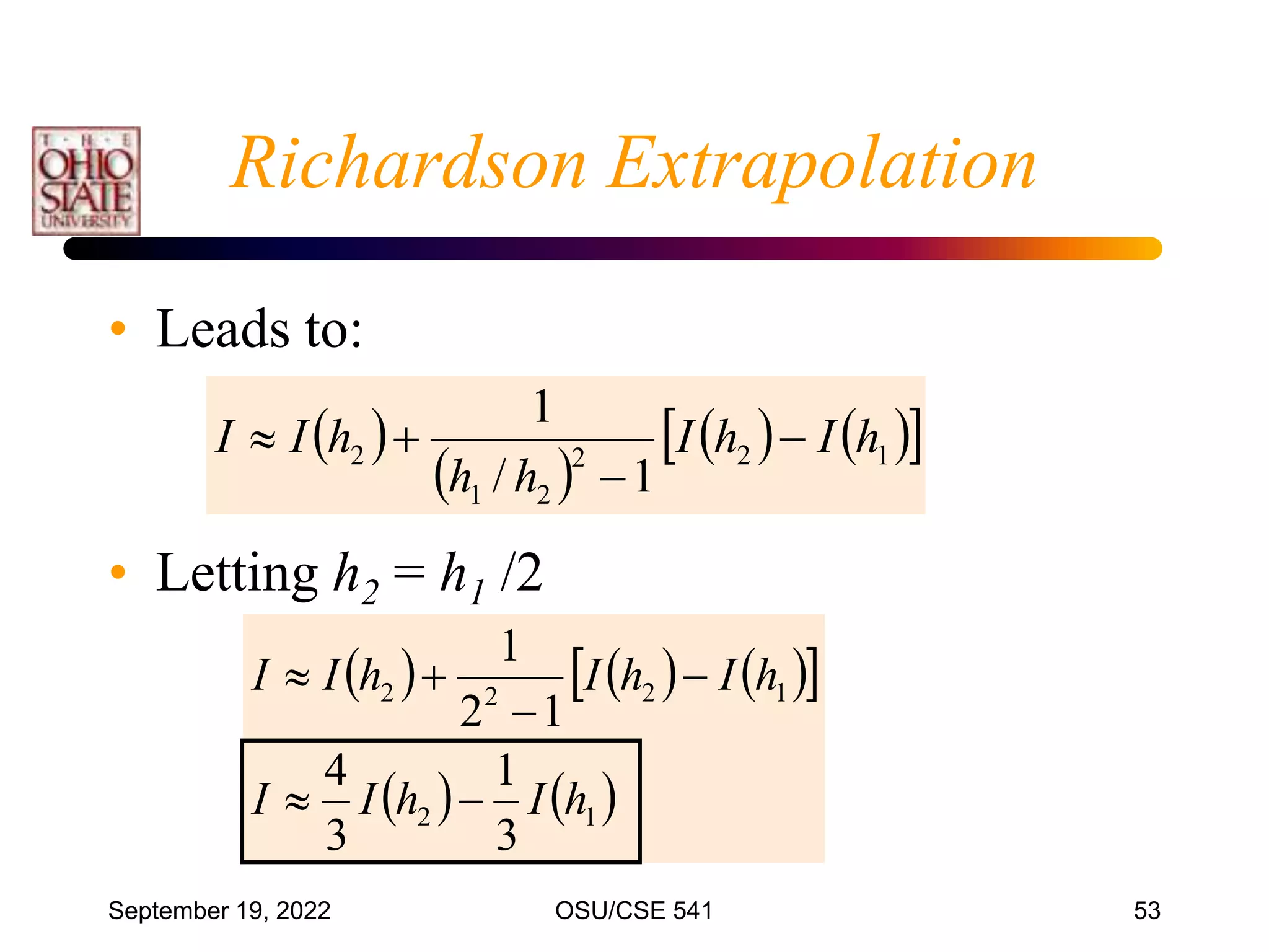
Richardson Extrapolation
• For example: Using (n = 2)
• where c is a constant
• Therefore:
2
2
2
1
2
1
h
h
h
E
h
E
f
ch
E
2
[error = O(h2)]
order of error in
trapezoidal rule](https://image.slidesharecdn.com/cis54107integration-220919040837-b4ac4cde/75/CIS541_07_Integration-ppt-50-2048.jpg)
![September 19, 2022 OSU/CSE 541 56
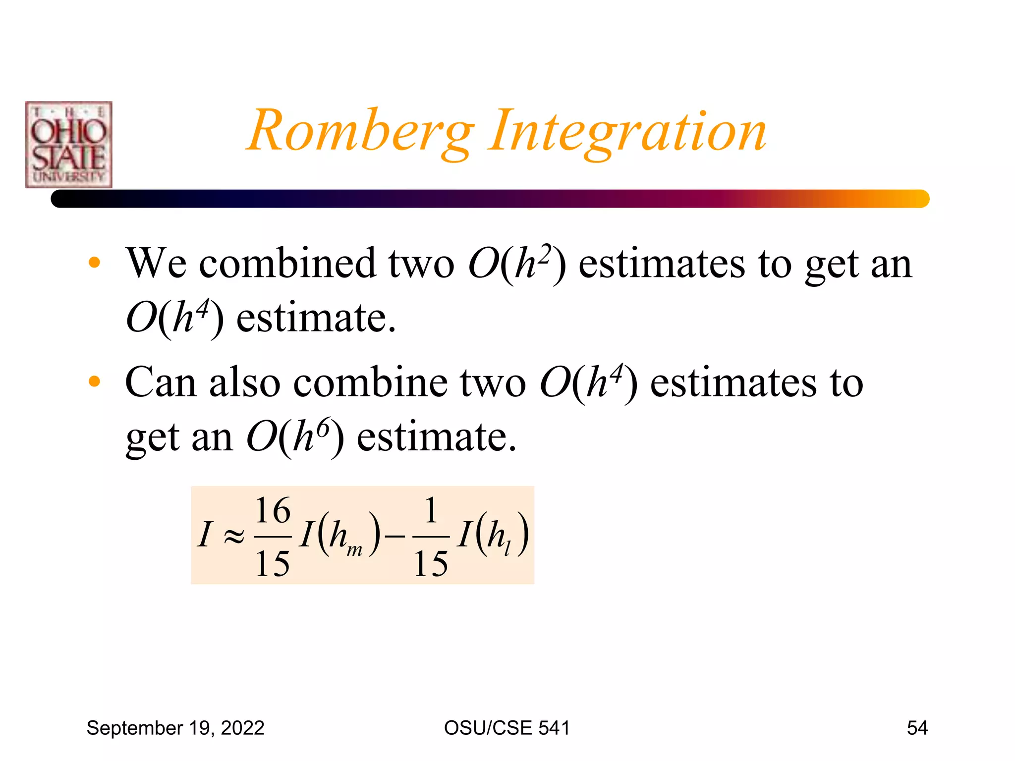
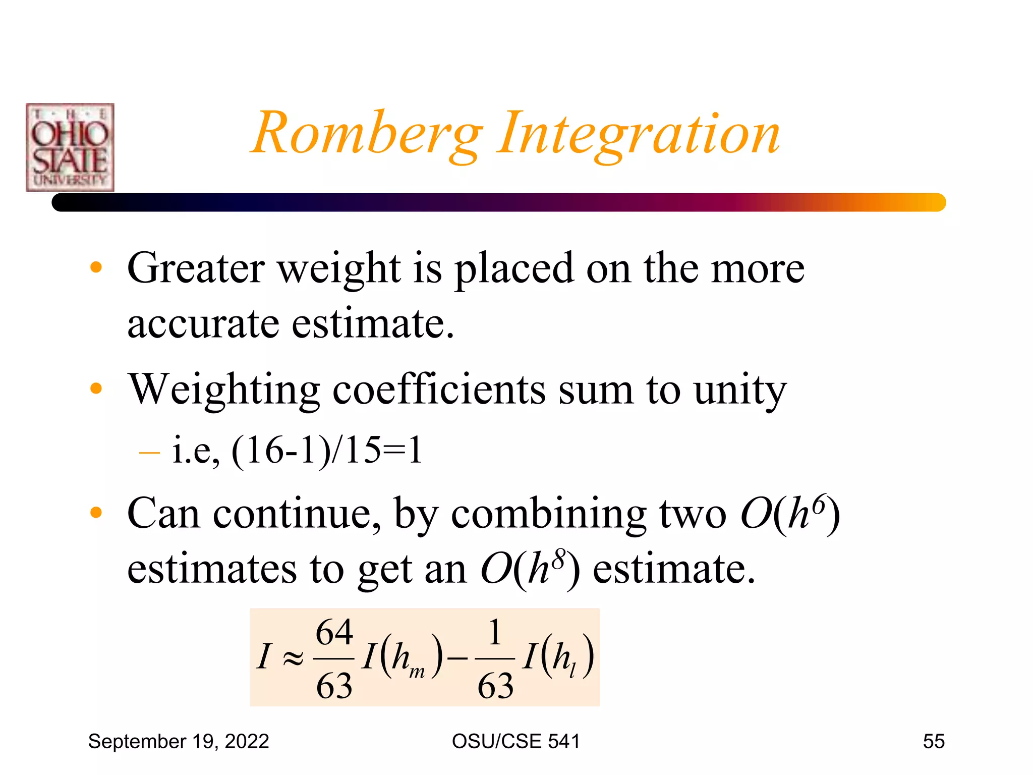
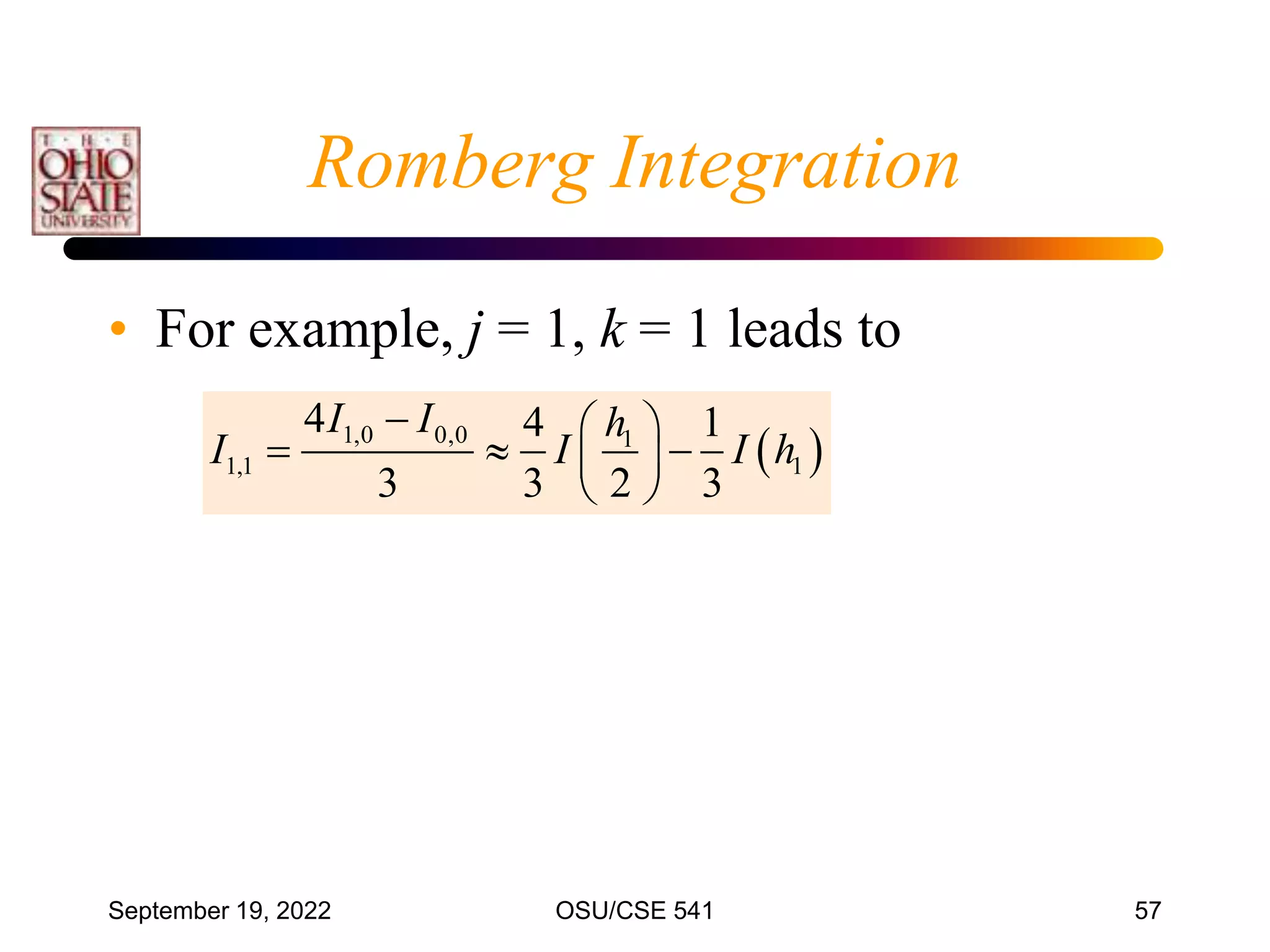
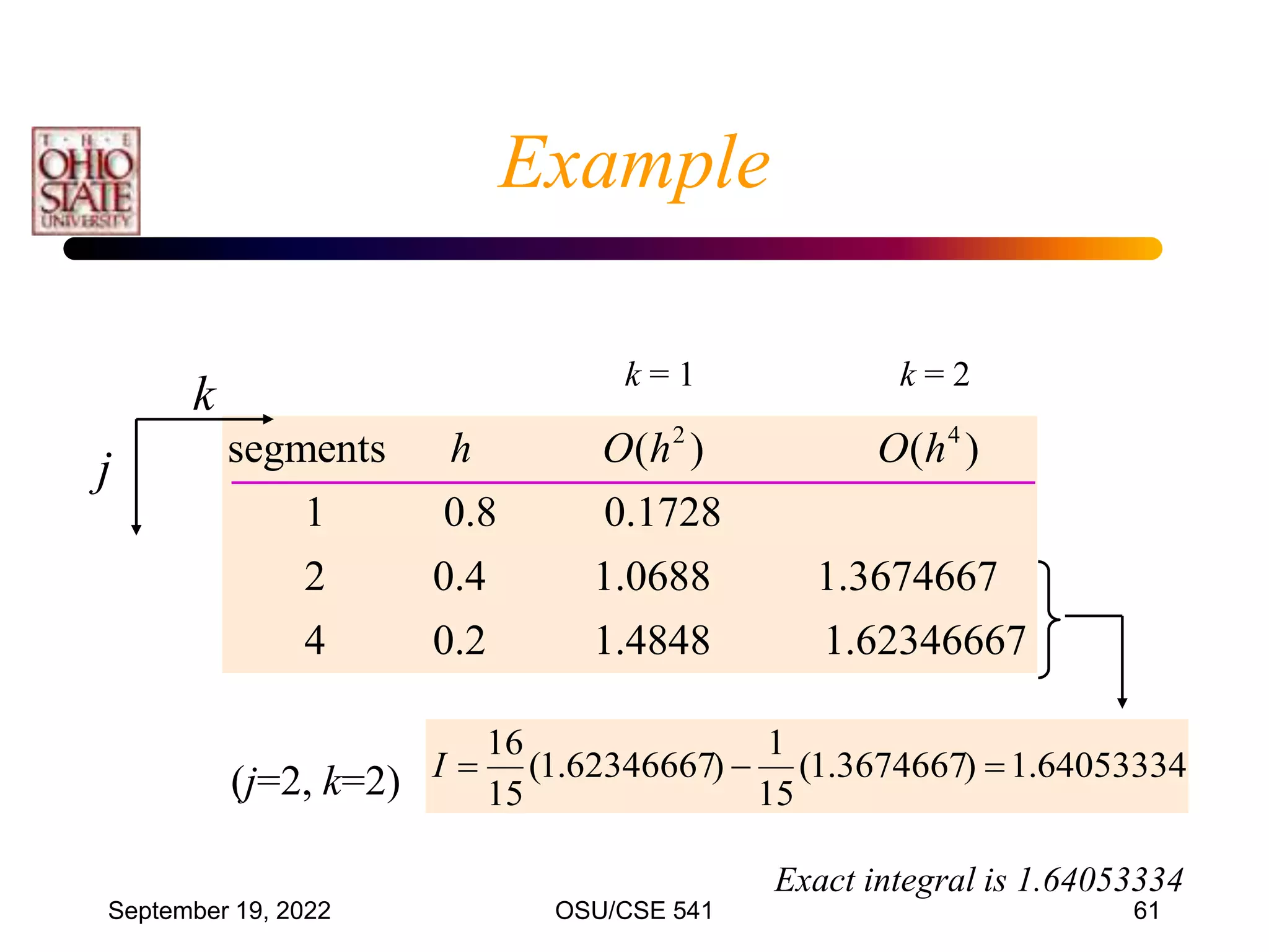
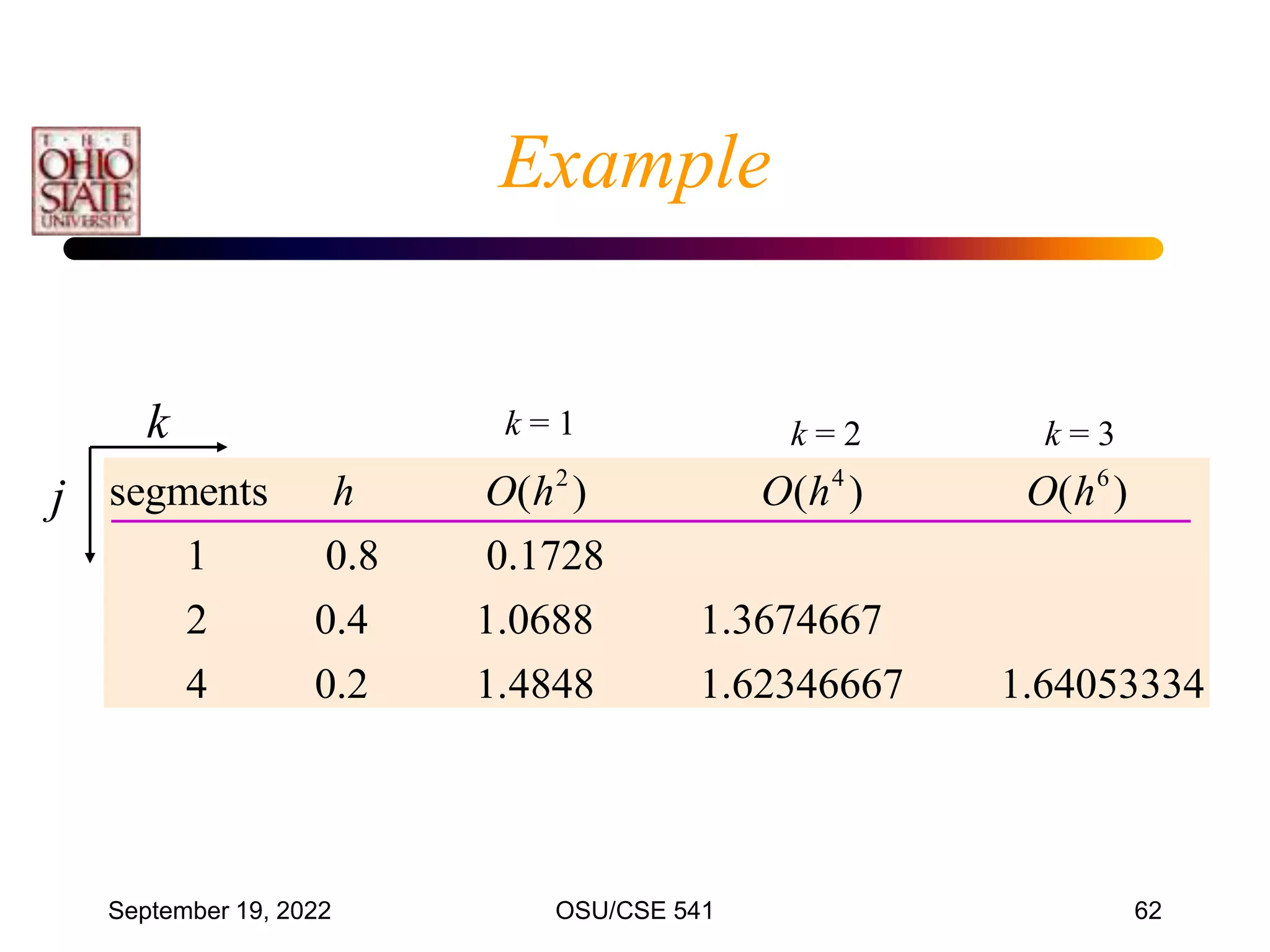
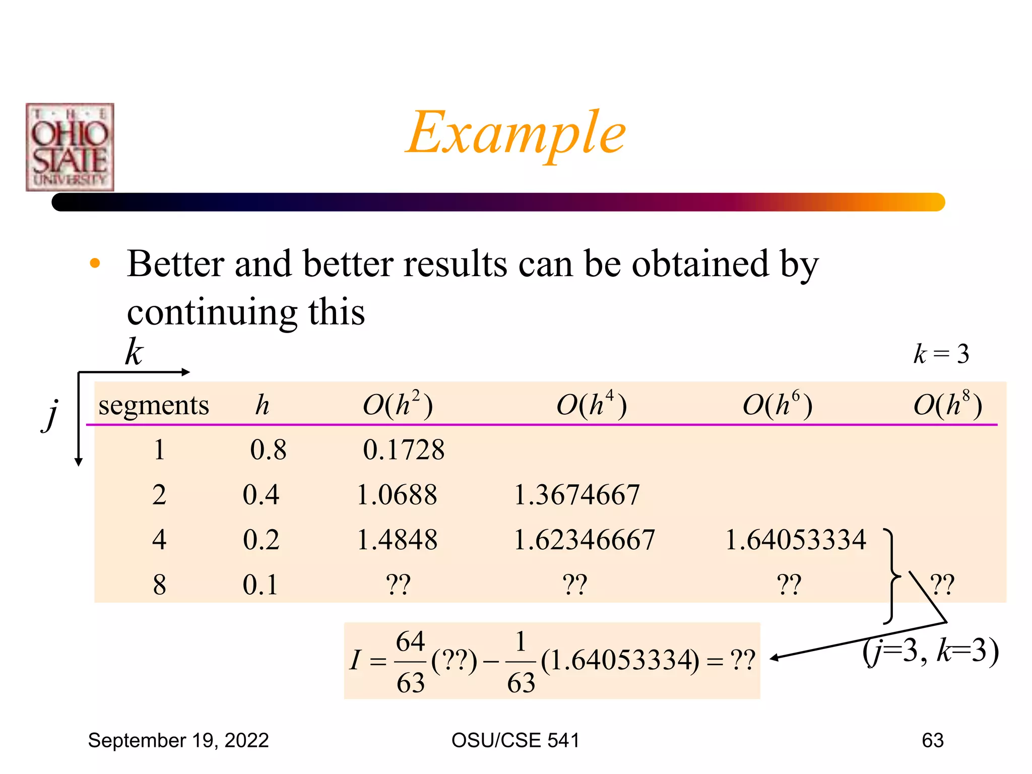
• General pattern is called Romberg Integration
– j : level of subdivision, j+1 has more intervals.
– k : level of integration, k = 1 is original trapezoid
estimate [O(h2)], k = 2 is improved [O(h4)], etc.
, 1,
, 1 , , 1,
4 1
4 1 4 1
k
j k j k
j k j k j k j k
k k
I I
I I I I
Romberg Integration](https://image.slidesharecdn.com/cis54107integration-220919040837-b4ac4cde/75/CIS541_07_Integration-ppt-56-2048.jpg)
![September 19, 2022 OSU/CSE 541 81
• If we use 4 segments instead of 1:
– x = [0.0 0.2 0.4 0.6 0.8]
0.2
b a
h
n
232
.
0
)
8
.
0
(
464
.
3
)
6
.
0
(
456
.
2
)
4
.
0
(
288
.
1
)
2
.
0
(
2
.
0
)
0
(
f
f
f
f
f
6234667
.
1
12
232
.
0
)
456
.
2
(
2
)
464
.
3
288
.
1
(
4
2
.
0
8
.
0
)
4
)(
3
(
)
8
.
0
(
)
6
.
0
(
4
)
4
.
0
(
2
)
2
.
0
(
4
)
0
(
0
8
.
0
3
2
4
1
5
,
3
,
1
2
6
,
4
,
2
0
f
f
f
f
f
n
x
f
x
f
x
f
x
f
a
b
I
n
n
i
n
j
j
i
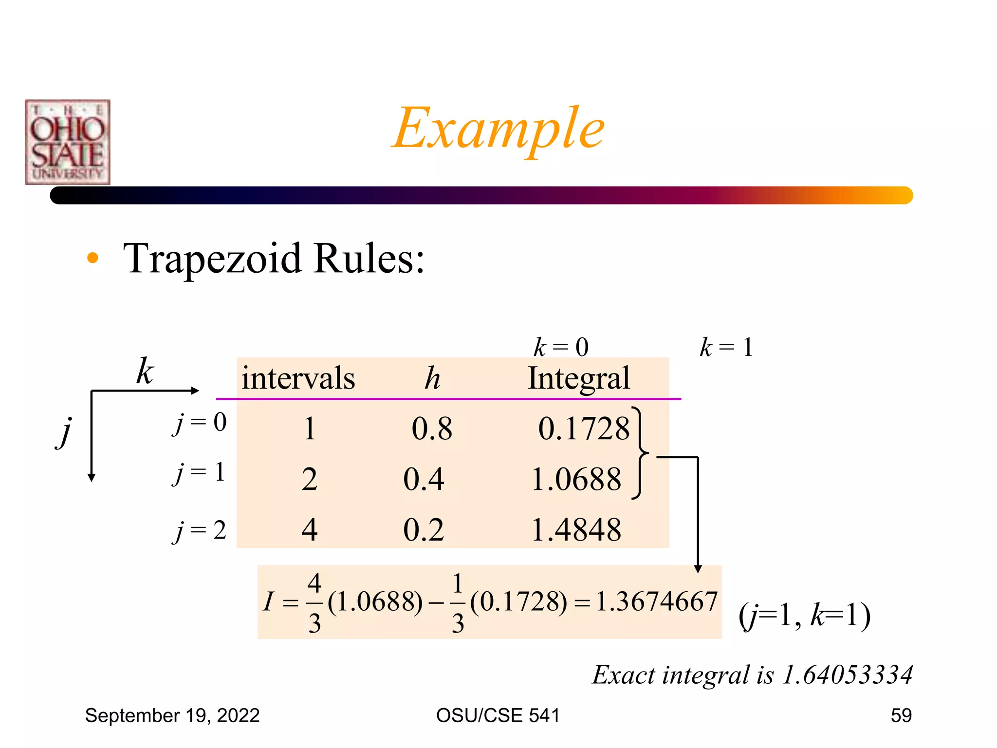
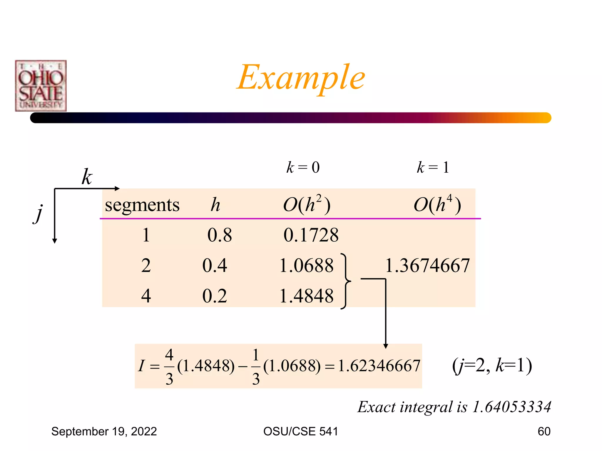
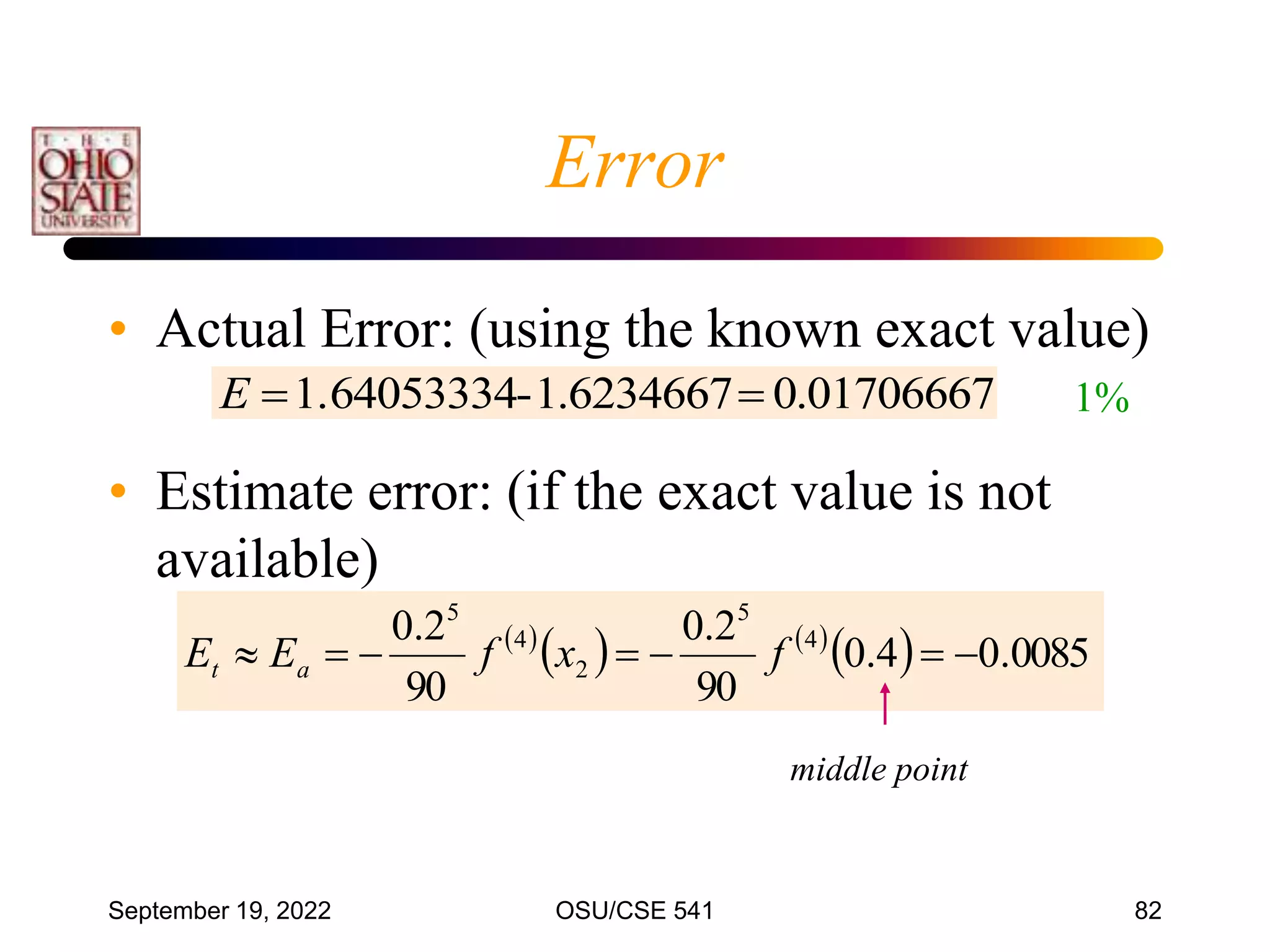
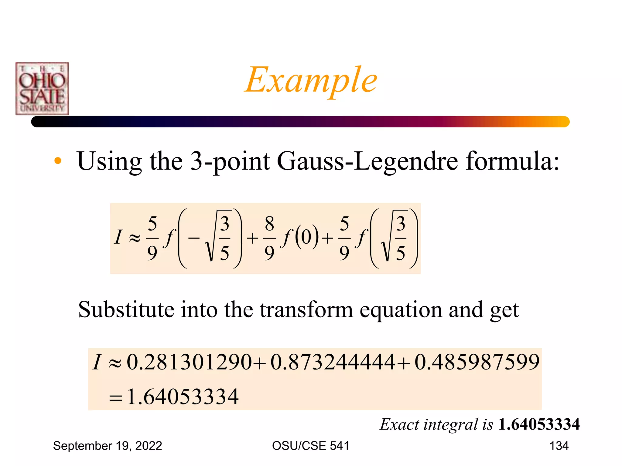
Exact integral is 1.64053334
Example Continued](https://image.slidesharecdn.com/cis54107integration-220919040837-b4ac4cde/75/CIS541_07_Integration-ppt-81-2048.jpg)


![September 19, 2022 OSU/CSE 541 117
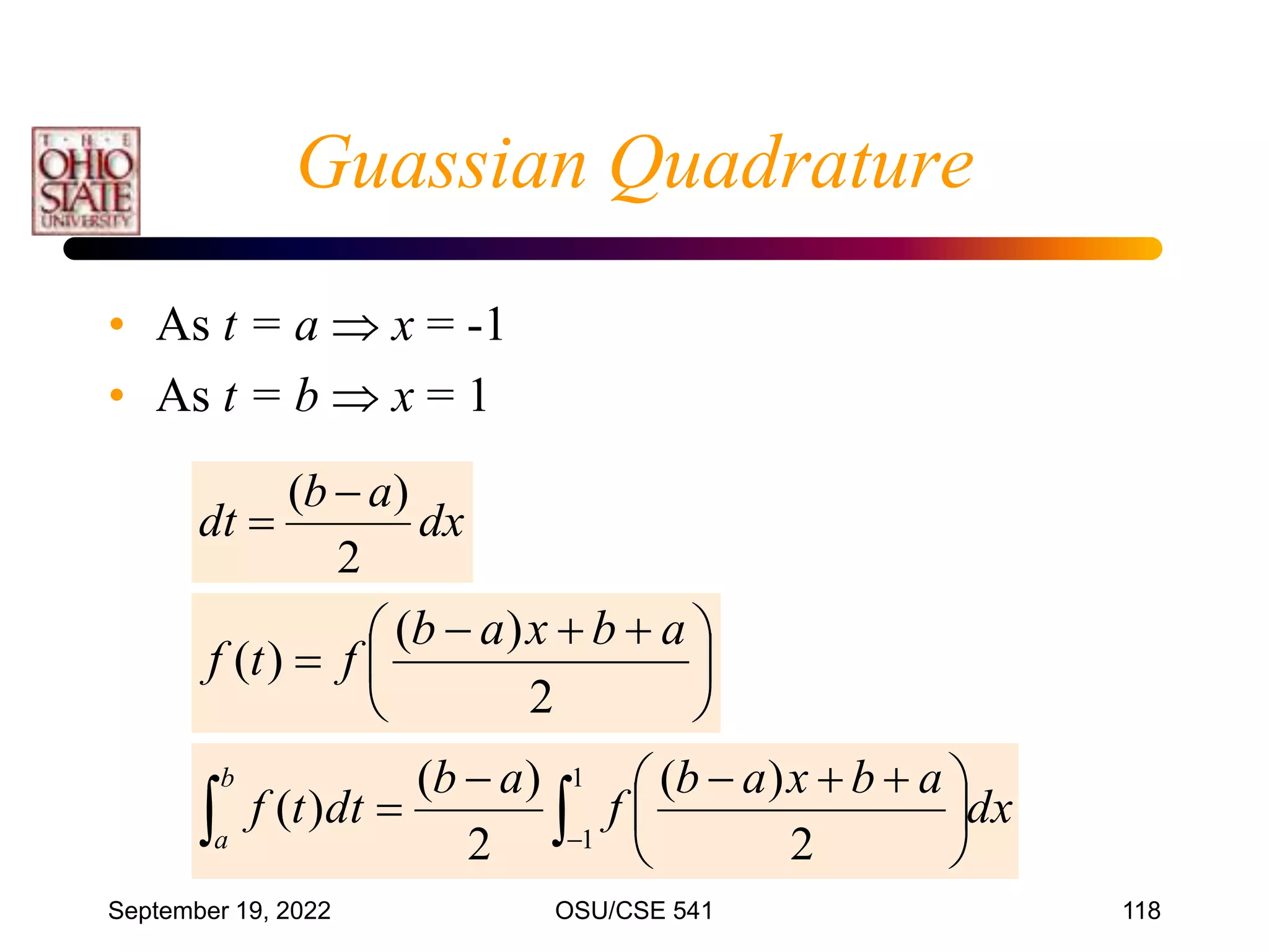
• Note that the interval is between –1 and 1
• For other intervals, a change of variables is used to
transfer the problem so that it utilizes the interval
[-1, 1]
• This is a linear transform, such that for t[a,b]:
• We have for x[-1,1]:
b
a
dt
t
f )
(
2
)
( a
b
x
a
b
t
a
b
a
b
t
x
2
Guassian Quadrature](https://image.slidesharecdn.com/cis54107integration-220919040837-b4ac4cde/75/CIS541_07_Integration-ppt-117-2048.jpg)
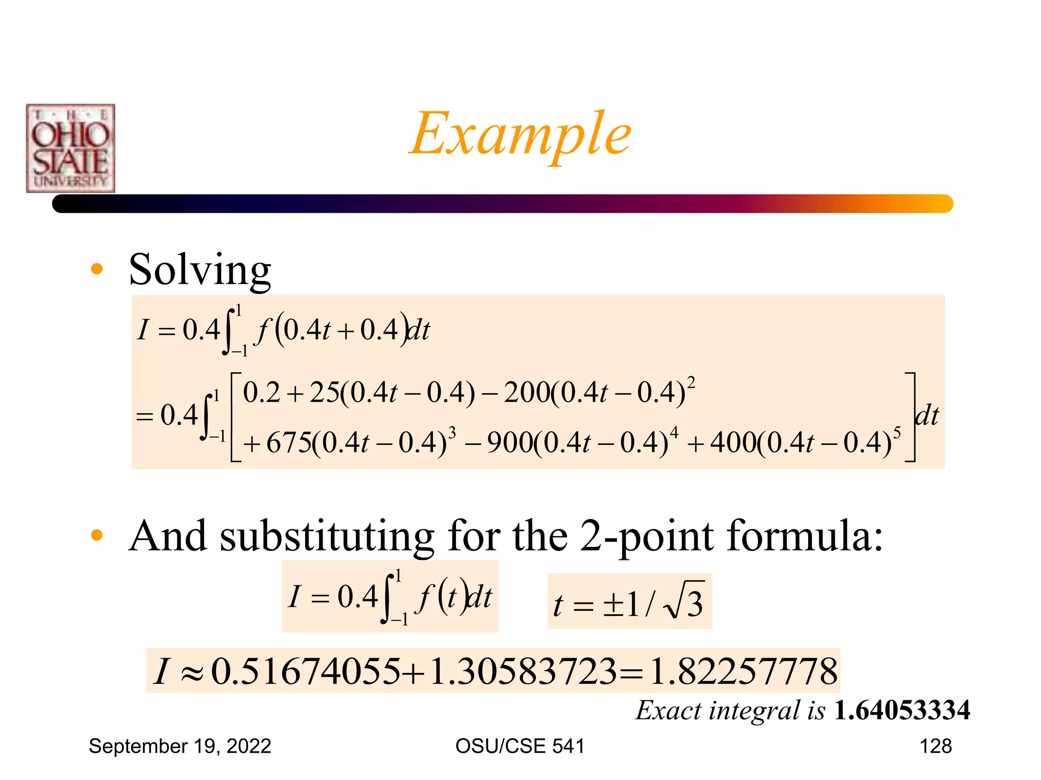
![September 19, 2022 OSU/CSE 541 127
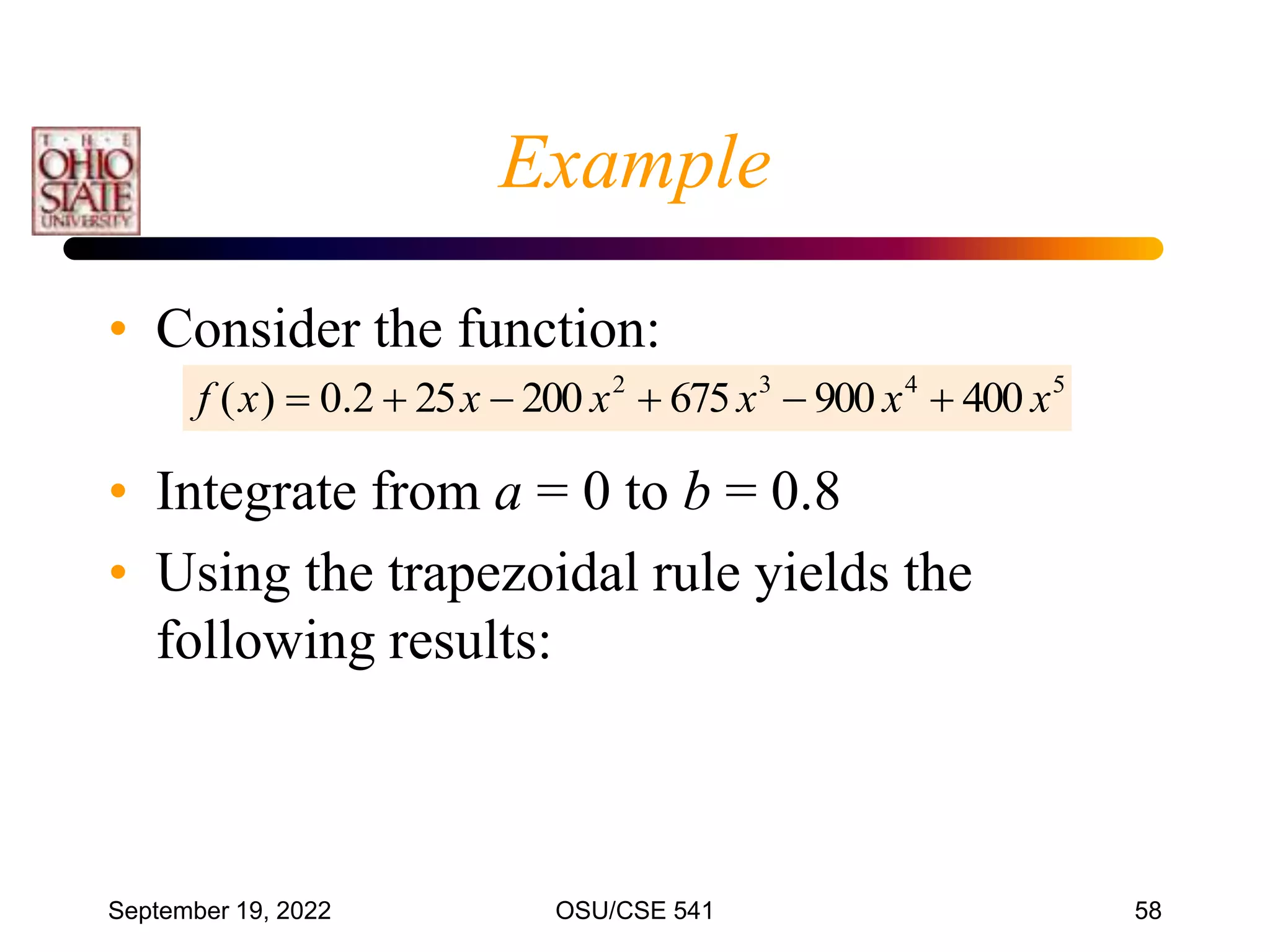
Example
5
4
3
2
400
900
675
200
25
2
.
0
)
( x
x
x
x
x
x
f
dx
a
b
x
a
b
f
a
b
dt
t
f
b
a
1
1 2
)
(
2
)
(
)
(
dt
t
f
dt
t
f
dx
x
f
I
1
1
1
1
8
.
0
0
4
.
0
4
.
0
4
.
0
2
0
8
.
0
)
0
8
.
0
(
2
)
0
8
.
0
(
)
(
• Integrate f(x) from a = 0 to b = 0.8
• Transform from [0, 0.8] to [-1, 1]](https://image.slidesharecdn.com/cis54107integration-220919040837-b4ac4cde/75/CIS541_07_Integration-ppt-127-2048.jpg)
![September 19, 2022 OSU/CSE 541 133
5
4
3
2
400
900
675
200
25
2
.
0
)
( x
x
x
x
x
x
f
Integrate from a = 0 to b = 0.8
Transform from [0, 0.8] to [-1, 1]
dt
t
t
t
t
t
dx
x
f
I
1
1 5
4
3
2
8
.
0
0
)
4
.
0
4
.
0
(
400
)
4
.
0
4
.
0
(
900
)
4
.
0
4
.
0
(
675
)
4
.
0
4
.
0
(
200
)
4
.
0
4
.
0
(
25
2
.
0
Example
replace -0.4 with +0.4](https://image.slidesharecdn.com/cis54107integration-220919040837-b4ac4cde/75/CIS541_07_Integration-ppt-133-2048.jpg)
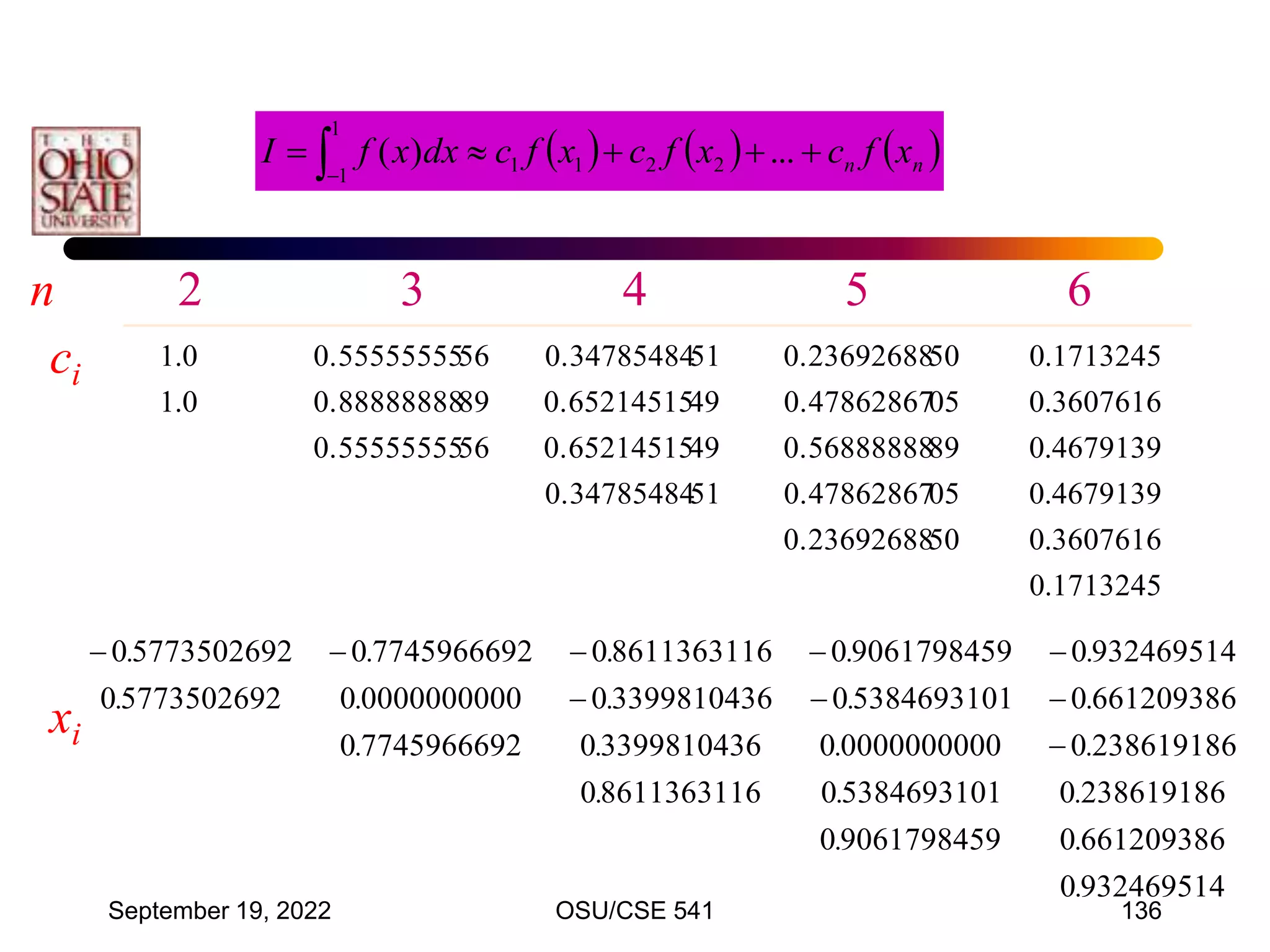
![September 19, 2022 OSU/CSE 541 135
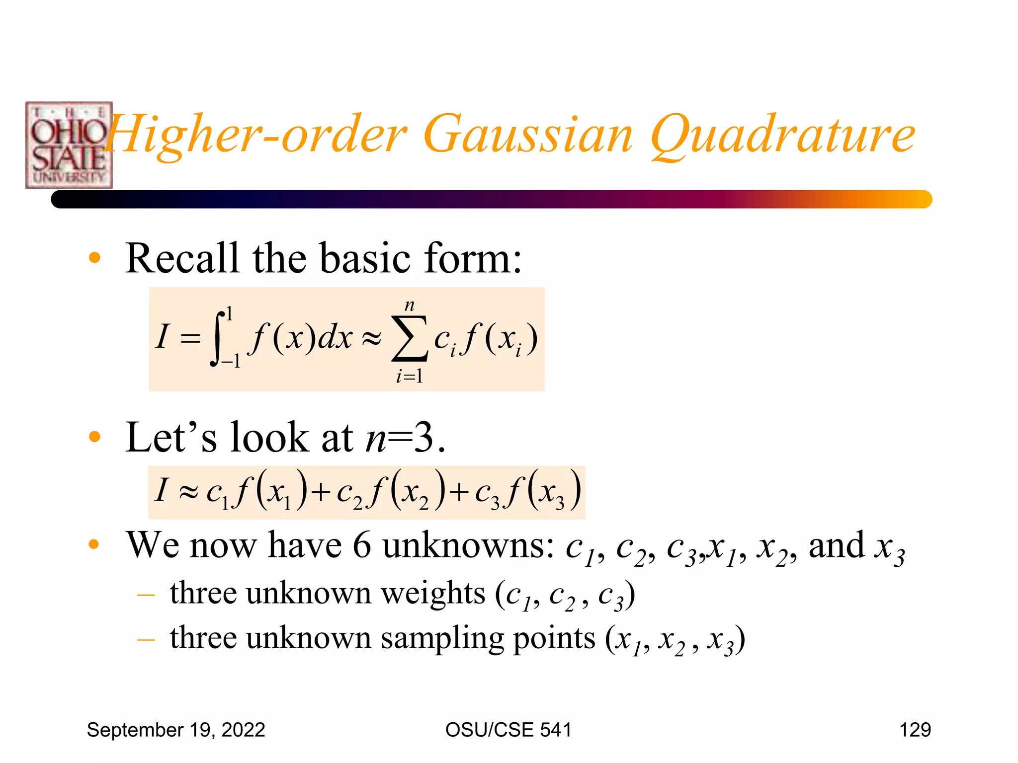
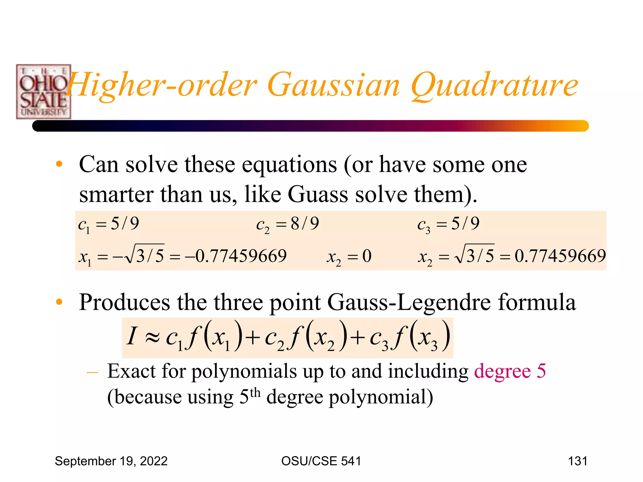
Can develop higher order Gauss-Legendre forms
using
n
n x
f
c
x
f
c
x
f
c
I
...
2
2
1
1
Values for c’s and x’s are tabulated
Use the same transformation to map interval onto
[-1, 1]
Gaussian Quadrature](https://image.slidesharecdn.com/cis54107integration-220919040837-b4ac4cde/75/CIS541_07_Integration-ppt-135-2048.jpg)