Download as PDF, PPTX


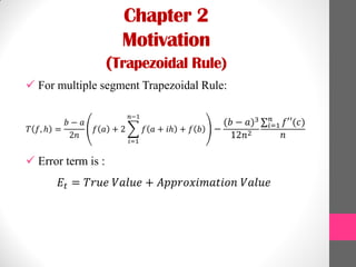
![Chapter 3
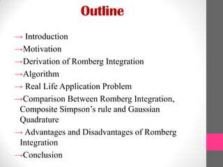
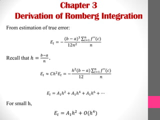
Derivation of Romberg Integration
(Error in Multiple Segment of Trapezoidal Rule)
𝐸𝑡 = −
(𝑏 − 𝑎)3
12𝑛2
𝑓′′(𝑐)𝑛
𝑖=1
𝑛
where 𝑐 ∈ [𝑎 + 𝑖 − 1 ℎ, 𝑎 + 𝑖ℎ] for each i.
𝑓′′(𝑐)𝑛
𝑖=1
𝑛
is the approximate average of f’’(x) in [a,b].
Because of that, we can say that :
𝐸𝑡 ≈ 𝛼
1
𝑛2](https://image.slidesharecdn.com/romberg-151219172120/85/Romberg-8-320.jpg)
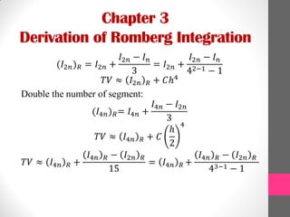

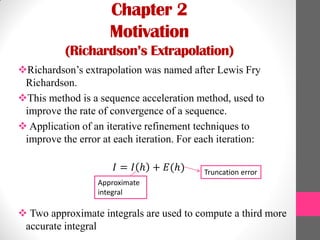
![Chapter 4
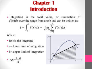
Algorithm
T approximate the integral 𝐼 = 𝑓 𝑥 𝑑𝑥
𝑏
𝑎
, select an integer n>0.
INPUT endpoints a,b; integer n
OUTPUT an array R. (Compute R by rows; only the last 2 rows are saved in storage).
Step 1: Set h=b-a;
𝑅1,1 = ℎ/2(𝑓 𝑎 + 𝑓 𝑏 )
Step 2: OUTPUT (𝑅1,1).
Step 3: For i =2,…….,n do Steps 4-8.
Step 4: Set 𝑅2,1 =
1
2
[𝑅1,1 + ℎ 𝑓(𝑎 + 𝑘 − 0.5 ℎ)].2 𝑖−2
𝑘=1
(Approximation from Trapezoidal method)
Step 5: For j=2,….., i
set 𝑅2,𝑗 = 𝑅2,𝑗−1 +
𝑅2,𝑗−1−𝑅1,𝑗−1
4 𝑗−1−1
. 𝐸𝑥𝑡𝑟𝑎𝑝𝑜𝑙𝑎𝑡𝑖𝑜𝑛 .
Steps 6: OUTPUT ((𝑅1,1) for j=1,2,……..i).
Step 7: Set h=h/2.
Step 8: For j=1,2,…..i set 𝑅1,𝑗. = 𝑅2,𝑗. (𝑈𝑝𝑑𝑎𝑡𝑒 𝑟𝑜𝑤 1 𝑜𝑓 𝑅)..
Step 9: STOP](https://image.slidesharecdn.com/romberg-151219172120/85/Romberg-14-320.jpg)
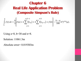

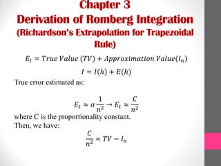
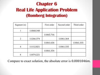
![Chapter 6
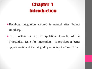
Real Life Application Problem
(Romberg Integration)
Step 1: Calculate the estimate of the integral using 1,2,4,8
subintervals using recursive integral:
𝑇 0 =
𝑏 − 𝑎
2
(𝑓 𝑎 + 𝑓 𝑏 )
𝑇 𝑗 =
𝑇(𝑗 − 1)
2
+ ℎ 𝑓[𝑥2𝑘−1]
2 𝑗−1
𝑘=1
j=1,2,3…
where ℎ =
𝑏−𝑎
2 𝑗 ,
𝑥 𝑘= 𝑥0 + 𝑘ℎ.
j T(j) Partition(𝟐𝒋)
0 118.68.348 1
1 11266.374 2
2 11112.821 4
3 11074.221 8
4 11065.933 16](https://image.slidesharecdn.com/romberg-151219172120/85/Romberg-17-320.jpg)
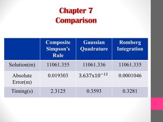


1) Romberg integration is a numerical method for approximating definite integrals based on Richardson extrapolation of the trapezoidal rule. It provides better approximations than the trapezoidal rule by reducing the true error through recursive calculations. 2) The derivation of Romberg integration involves applying Richardson's extrapolation to the error estimation of the trapezoidal rule. This allows computing a more accurate integral using the results from two less accurate integrals. 3) An example application calculates the volume of water in a tank using Romberg integration, Composite Simpson's rule, and Gaussian quadrature. Romberg integration provided the most accurate result with less computation time compared to the other methods.