Downloaded 40 times

![INTEGRATION TECHNIQUES
9
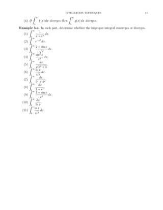
Brief Summary of Integration Techniques.
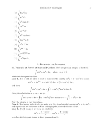
ˆ
ˆ
• Integration by Substitution:
f (u(x))u (x) dx = f (u) du
What to look for
– Compositions of the form f (u(x)), where the integrand also contains u (x); for
example,
ˆ
ˆ
ˆ
2
2
2x cos(x ) dx = cos(x )2x dx = cos udu.
– Compositions of the form f (ax + b); for example,
ˆ
ˆ
x
u−1
√
√ du.
dx =
u
x+1
´
´
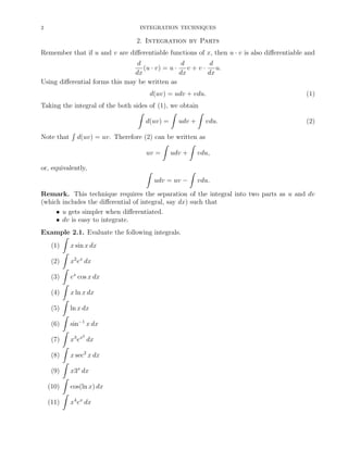
• Integration by Parts: u dv = uv − v du
What to look for: products of different types of functions: xn , cos x, ex ; for example,
ˆ
ˆ
2x cos x dx = x sin x − sin x dx.
• Trigonometric Substitutions:
What to look √
for:
– Terms like a2 − x2 : Let x = a sin θ, − π ≤ θ ≤ π , so that dx = a cos θ dθ and
2
2
√
a2 − x2 = a2 − a2 sin2 θ = a cos θ; for example,
ˆ
ˆ
x2
√
dx = sin2 θ dθ.
2
1−x
√
– Terms like x2 + a2 : Let x = a tan θ, − π < θ < π , so that dx = a sec2 θ dθ and
2
2
√
√
x2 + a2 = a2 tan2 θ + a2 = a sec θ; for example,
ˆ
ˆ
x3
√
dx = 27 tan3 θ sec θ dθ.
2+9
x
√
2 − a2 : Let x = a sec θ, for θ ∈ [0, π ) ∪ ( π , π], so that dx =
– Terms like x
2
2
√
√
a sec θ tan θ dθ and x2 − a2 = a2 sec2 θ − a2 = a tan θ; for example,
ˆ
ˆ
√
3
2 − 4 dx = 32
x x
sec4 θ tan2 θ dθ.
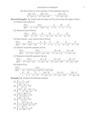
• Partial Fractions:
What to look for: rational functions, for example,
ˆ
ˆ
ˆ
x+2
x+2
A
B
dx =
dx =
+
2 − 4x + 3
x
(x − 1)(x − 3)
x−1 x−3
dx.](https://image.slidesharecdn.com/integrationtechniques-140106221701-phpapp02/85/Integration-techniques-9-320.jpg)
![10
INTEGRATION TECHNIQUES
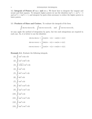
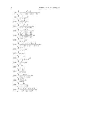
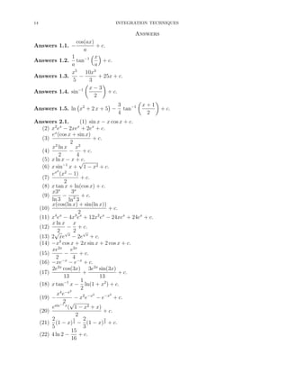
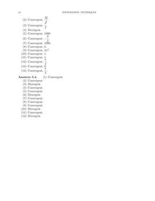
5. Improper Integrals
ˆ
2
Example 5.1. Evaluate
−1
1
dx.
x2
When studying the definite integrals, we required two things. First, the domain of integration
(from a to b) [a, b], be finite. Second, function is finite on the domain of integration.
Question: What happens if the domain of integration is infinite? What if function becomes
infinite in the domain of integration?
Answer: Improper integration!
The integrals of type described above are called improper integrals. If the limits exist, we
evaluate them with the following definitions
(1) If f is continuous on [a, ∞), then
ˆ ∞
ˆ b
f (x) dx = lim
f (x) dx.
b→∞
a
a
(2) If f is continuous on (−∞, b], then
ˆ b
ˆ b
f (x) dx = lim
f (x) dx.
a→−∞
−∞
a
(3) If f is continuous on [a, b) then
ˆ b
ˆ c
f (x) dx = lim
f (x) dx.
−
c→b
a
a
(4) If f is continuous on (a, b] then
ˆ b
ˆ b
f (x) dx = lim
f (x) dx.
+
c→a
a
c
In each case, if the limit exists and is finite we say that the improper integral converges and
the limit is the value of the improper integral. Otherwise the improper integral diverges.
Similarly, if f becomes infinite at an interior point d ∈ [a, b], then
ˆ b
ˆ d
ˆ b
f (x) dx =
f (x) dx +
f (x) dx.
a
a
d
This integral (on [a, b]) converges if both integrals (on [a, d] and on [d, b]) converges. Otherwise,
the integral from a to b diverges.
ˆ
ˆ
∞
a
Finally, if f is continuous on (−∞, ∞) and if
ˆ ∞
f (x) dx converges and its value is
−∞
ˆ
ˆ
∞
−∞
f (x) dx +
−∞
f (x) dx both converge, then
a
ˆ
a
f (x) dx =
−∞
f (x) dx and
∞
f (x) dx.
a
If either one or both of the integrals on the right-hand side of this equation diverge, the integral
diverges.
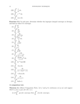
Example 5.2. In each part, determine whether the improper integral converges or diverges,
and find its value if it converges.](https://image.slidesharecdn.com/integrationtechniques-140106221701-phpapp02/85/Integration-techniques-10-320.jpg)
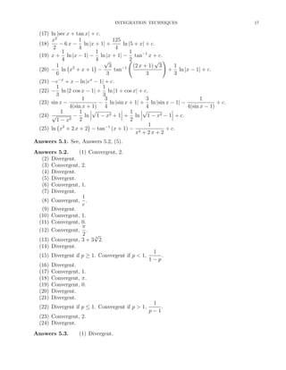

(1) The document discusses various integration techniques including: review of integral formulas, integration by parts, trigonometric integrals involving products of sines and cosines, trigonometric substitutions, and integration of rational functions using partial fractions. (2) Examples are provided to demonstrate each technique, such as using integration by parts to evaluate integrals of the form ∫udv, using trigonometric identities to reduce powers of trigonometric functions, and using partial fractions to break down rational functions into simpler fractions. (3) The key techniques discussed are integration by parts, trigonometric substitutions to transform integrals involving quadratic expressions into simpler forms, and partial fractions to decompose rational functions for integration. Various examples illustrate the