The document discusses the beta and gamma functions, addressing their definitions, properties, transformations, and relations. It includes integrals, the symmetry of these functions, and their applications in solving mathematical problems. The content features proofs, evaluations, and examples relevant to these mathematical concepts.

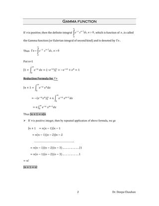
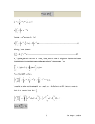
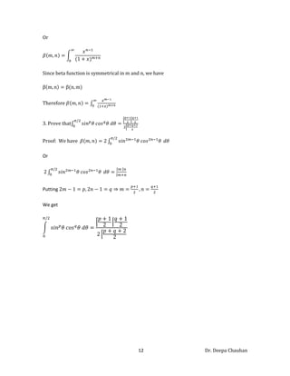
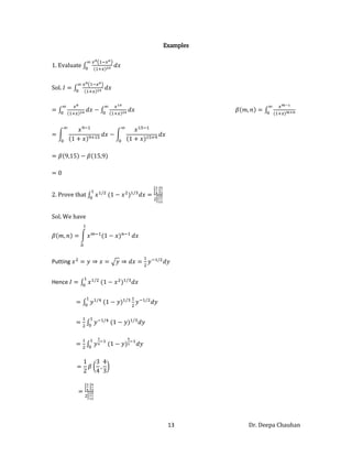
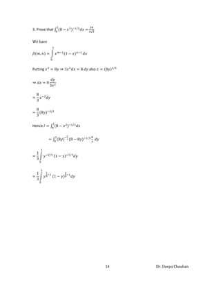
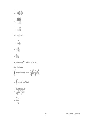
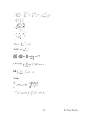
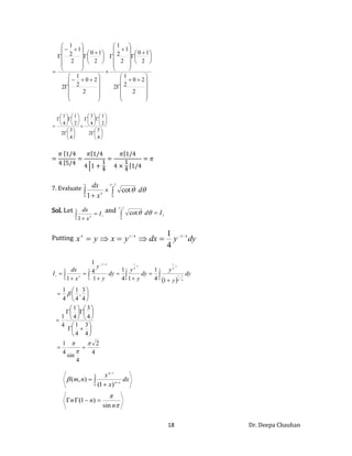
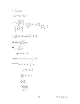
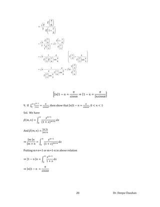
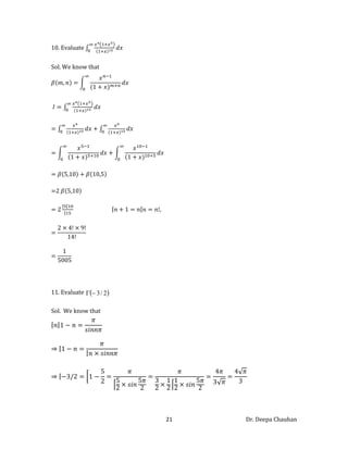
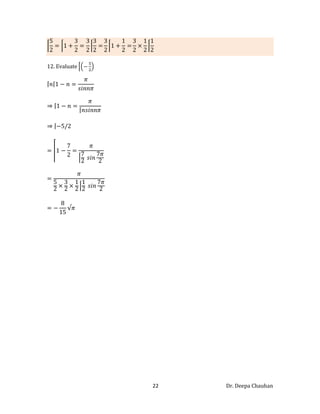
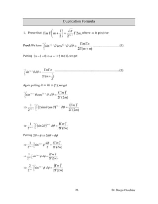
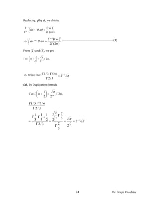
1. 1
Beta & Gamma Functions
By
Dr. Deepa Chauhan
Associate Professor,
Applied Science & Humanities Department,
Axis Institute of Technology, Kanpur

2. 2 Dr. Deepa Chauhan
Gamma function
If nis positive, then the definite integral 




0
1
0
, n
dx
x
e n
x
, which is function of n, is called
the Gamma function (or Eulerian integral of second kind) and is denoted by n
 .
Thus 






0
1
0
, n
dx
x
e
n n
x
Put n=1
Reduction Formula for n

Thus
 If nis positive integer, then by repeated application of above formula, we ge
………………………………………………..

3. 3 Dr. Deepa Chauhan
Value of 






2
1
If 






0
1
0
, n
dx
x
e
n n
x
dt
t
e t












0
2
/
1
2
1
Putting 2
x
t  so that xdx
dt 2

)
1
(
..........
..........
..........
..........
..........
..........
..........
..........
..........
2
2
.
1
.
2
1
0
0
2
2
dx
e
xdx
x
e x
x















Writing y for x, we have
…………………………………………………………………………………………………………..(2)
If )
(x
f and )
(x
g are functions of x and y only, and the limits of integration are constants then
double integration can be represented as a product of two integrals. Thus
  

d
c
b
a
b
a
d
c
dy
y
g
dx
x
f
dy
dx
y
g
x
f )
(
)
(
)
(
)
(
From (1) and (2) we have:



 





















0 0
)
(
0
0
2
2
2
2
2
4
4
2
1
dy
dx
e
dy
e
dx
e y
x
y
x
Changing to polar coordinates with 

 rdrd
dxdy
r
y
r
x 

 ,
sin
,
cos ; therefore r varies
from 0 to  and  from 0 to
2


 
 



























2
/
0
0
2
/
0
2
/
0
0
2
2
2
1
4
4
2
1 2
2

 



 d
d
e
rdrd
e r
r
Hence 








2
1

4. 4 Dr. Deepa Chauhan

5. 5 Dr. Deepa Chauhan
1. Prove that
Sol. 






0
1
0
, n
dx
x
e
n n
x
Let
2. Evaluate
Sol. Let

6. 6 Dr. Deepa Chauhan
3. Prove that
Sol.
Let
and
Let

7. 7 Dr. Deepa Chauhan
Transformations of Gamma Functions
1. dx
x
e
k
n n
kx
n






0
1
Sol. Let kx=t, kdx=dt
Then
Or
Proof: we have

















0
1
0
1
1
0
1
dy
y
e
k
dy
k
y
k
e
dx
x
e
n
n
ky
n
n
n
ky
n
x
kdy
dx
ky
x
Put



dx
x
e
k
n n
kx
n







0
1
2. Show that 0
;
1
log
1
0
1














 

n
dx
x
n
n
Proof. Let
When
When
3. Show that
Sol. Let
When

8. 8 Dr. Deepa Chauhan
When
Beta Function
The definite integral is called the Beta function and is
denoted by .
Thus
Beta function is also called the Eulerian Integral of the first kind.
Symmetry of Beta function
Since
Therefore
Hence

9. 9 Dr. Deepa Chauhan
Relation between Beta and Gamma Functions
  0
,
0
;
, 





 n
m
n
m
n
m
n
m

Proof:
We know that   dt
t
e
m m
t






0
1
Putting 2
x
t  so that xdx
dt 2

  dx
x
e
m m
x 1
2
0
2
2 





Similarly
  dy
y
e
n n
y 1
2
0
2
2 





Now,
  dy
y
e
dx
x
e
n
m n
y
m
x 1
2
0
1
2
0
2
2
2
2 






 



  dy
dx
y
x
e
n
m n
m
y
x 1
2
0
1
2
0
)
( 2
2
4 





 



Changing to polar coordinates with 

 rdrd
dxdy
r
y
r
x 

 ,
sin
,
cos ;
therefore r varies from 0 to and  from 0to
2


10. 10 Dr. Deepa Chauhan
  dy
dx
y
x
e
n
m n
m
y
x 1
2
0
1
2
0
)
( 2
2
4 





 



 









2
/
0
1
2
1
2
1
)
(
2
0
sin
cos
4
2



 drd
r
e
n
m n
m
n
m
r
 







2
/
0
1
)
(
2
0
1
2
1
2 2
sin
cos
4



 dr
r
e
d n
m
r
n
m





 








2
)
(
2
)
,
(
4
n
m
n
m

n
m
n
m 

 (
)
,
(

 
n
m
n
m
n
m





 ,

Let
Therefore

11. 11 Dr. Deepa Chauhan
Transformations of Beta Functions
1.
Proof. We have
Put
When
When
2.
Proof: We know that
(1)
Put
Also, when
And when
Thus, from (1)

12. 12 Dr. Deepa Chauhan
Or
Since beta function is symmetrical in m and n, we have
Therefore
3. Prove that
Proof: We have
Or
Putting
We get

13. 13 Dr. Deepa Chauhan
Examples
1. Evaluate
Sol.
2. Prove that
Sol. We have
Putting
Hence

14. 14 Dr. Deepa Chauhan
3. Prove that
We have
Putting also
Hence

15. 15 Dr. Deepa Chauhan
4. Evaluate
Sol. We have

16. 16 Dr. Deepa Chauhan
5. Using beta and gamma functions, evaluate



0
4
1 x
dx
Sol. We have
Putting dy
y
dx
y
x
y
x 4
/
3
4
/
1
4
4
1 






17. 17 Dr. Deepa Chauhan
 
4
2
4
sin
4
1
4
3
4
1
4
3
4
1
4
1
4
3
,
4
1
4
1
1
4
1
1
4
1
1
4
1
1 0 4
3
4
1
1
4
1
0
1
4
1
0
4
/
3
0
4











































 











dy
y
y
dy
y
y
dy
y
y
x
dx
I



n
n
n
dx
x
x
n
m n
m
m
sin
)
1
(
)
1
(
)
,
(
0
1





 



6. Prove that 



 

2
/
0
2
/
0
sin
sin
dx
x
x
dx
Sol.

 
2
/
0
2
/
0
sin
sin


dx
x
x
dx
We have

 

 2
/
0
0
2
1
2
/
0
0
2
1
cos
sin
cos
sin


dx
x
x
dx
x
x

18. 18 Dr. Deepa Chauhan




















 





































 

















2
2
0
2
1
2
2
1
0
2
1
2
1
2
2
0
2
1
2
2
1
0
2
1
2
1












































4
5
2
2
1
4
3
4
3
2
2
1
4
1
7. Evaluate

 

 2
/
0
0
4
cot
1


 d
x
dx
Sol. Let
1
0
4
1
I
x
dx




and
2
2
/
0
cot I
d 




Putting dy
y
dx
y
x
y
x 4
/
3
4
/
1
4
4
1 





 
4
2
4
sin
4
1
4
3
4
1
4
3
4
1
4
1
4
3
,
4
1
4
1
1
4
1
1
4
1
1
4
1
1 0 4
3
4
1
1
4
1
0
1
4
1
0
4
/
3
0
4
1











































 











dy
y
y
dy
y
y
dy
y
y
x
dx
I



n
n
n
dx
x
x
n
m n
m
m
sin
)
1
(
)
1
(
)
,
(
0
1





 




19. 19 Dr. Deepa Chauhan


2
/
0
2
cot


 d
I



2
/
0
2
/
1
2
/
1
sin
cos



 d
2
4
sin
2
1
2
4
1
1
4
1
1
2
4
3
4
1
2
2
2
1
2
1
2
2
1
2
1
2
1
2
1



















































































4
2
4
2
cot
1
2
2
/
0
0
4











 


d
x
dx
8. Evaluate 

1
0
3
3
1
dx
x
x
Sol.



1
0
3
3
1
dx
x
x
I
dx
x
x 2
/
1
3
1
0
2
/
3
)
1
( 

 
Putting dt
t
dx
t
x
t
x 3
/
2
3
/
1
3
3
1 





Therefore, dt
t
t
t
I 3
/
2
2
/
1
1
0
2
/
1
3
1
)
1
( 


 
dt
t
t 2
/
1
1
0
6
/
1
)
1
(
3
1 


 
dt
t
t
1
2
1
1
0
1
6
5
)
1
(
3
1 


 







2
1
,
6
5
3
1























3
4
2
1
6
5
3
1

20. 20 Dr. Deepa Chauhan
















3
1
1
6
5
3








































































































6
1
3
2
3
6
sin
6
1
3
sin
3
2
1
3
sin
3
2
3
1
6
sin
6
1
3
1
1
3
1
6
1
1
3
1
3
1
6
5
3













9. If , then show that
Sol. We have
And
Putting m+n=1 or m=1-n in above relation

21. 21 Dr. Deepa Chauhan
10. Evaluate
Sol. We know that
=2
11. Evaluate  
2
/
3


Sol. We know that

22. 22 Dr. Deepa Chauhan
12. Evaluate

23. 23 Dr. Deepa Chauhan
Duplication Formula
1. Prove that ,
2
2
2
1
1
2
m
m
m m










 
 where m is positive
Proof: We have
)
(
2
cos
sin 1
2
2
/
0
1
2
n
m
n
m
d
n
m







 



Putting 2
/
1
0
1
2 


 n
n in (1), we get
)
2
1
(
2
sin
2
/
0
1
2







m
m
d
m 



.(2)
Again putting m
n  in (1), we get
 
)
2
(
2
cos
sin
2
1
2
2
/
0
1
2
m
m
d
m
m





 



 
 
)
2
(
2
cos
sin
2
2
1
2
2
/
0
1
2
1
2
m
m
d
m
m



 






 
 
)
2
(
2
2
sin
2
1
2
2
/
0
1
2
1
2
m
m
d
m
m



 





Putting 


 d
d 

 2
2
 
)
2
(
2
2
sin
2
1
2
0
1
2
1
2
m
m
d
m
m



 





 
)
2
(
2
sin
2
1
2
0
1
2
2
m
m
d
m
m



 




 
)
2
(
2
sin
2
2
2
2
/
0
1
2
2
m
m
d
m
m



 





24. 24 Dr. Deepa Chauhan
Replacing  by  , we obtain,
 
)
2
(
2
sin
2
2
2
2
/
0
1
2
2
m
m
d
m
m








 
)
2
(
2
2
sin
2
1
2
2
/
0
1
2
m
m
d
m
m






 


From (2) and (3), we get
,
2
2
2
1
1
2
m
m
m m










 

13. Prove that 
3
/
1
2
3
/
2
6
/
5
3
/
1




Sol. By Duplication formula
,
2
2
2
1
1
2
m
m
m m










 




3
/
1
3
1
1
3
2
2
2
3
2
3
2
2
3
/
2
2
1
3
1
3
1
3
/
2
6
/
5
3
/
1














