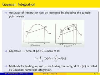
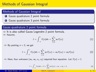
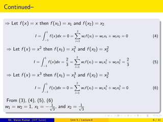
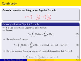
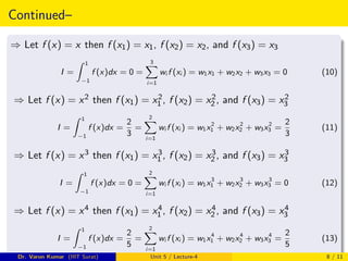
This document discusses Gaussian numerical integration techniques. It describes the Gauss quadrature 2-point and 3-point formulas for numerical integration. The 2-point formula uses two sample points with equal weights of 1 to calculate the integral. The 3-point formula uses three sample points and weights of 5/9, 8/9 and 5/9 to yield more accurate integration over an interval. The document also explains how to apply these formulas when the integral limits differ from [-1,1].

1. Gaussian Numerical Integration
Dr. Varun Kumar
Dr. Varun Kumar (IIIT Surat) Unit 5 / Lecture-4 1 / 11

2. Outlines
1 Newton’s Cotes Integration
2 Gaussian Integration
3 Gauss Quadrature 2 Point Formula
4 Gauss Quadrature 3 Point Formula
Dr. Varun Kumar (IIIT Surat) Unit 5 / Lecture-4 2 / 11

3. Newton’s Cotes Integration
Newton’s Cotes Integration
⇒ Trapezoidal rule
⇒ Simpson’s 1
3rd rule
⇒ Simpson’s 3
8th rule
⇒ Romberg’s Integration
Important points
⇒ Above rules are derived from Newton’s divide difference interpolation.
⇒ In all the rules range of integral is divide into equally space.
Dr. Varun Kumar (IIIT Surat) Unit 5 / Lecture-4 3 / 11

4. Gaussian Integration
⇒ Accuracy of integration can be increased by choosing the sample
point wisely.
⇒ Objective → Area of (A+C)=Area of B.
I =
Z 1
−1
f (x)dx =
n
X
i=1
wi f (xi )
⇒ Methods for finding wi and xi for finding the integral of f (x) is called
as Gaussian numerical integration.
Dr. Varun Kumar (IIIT Surat) Unit 5 / Lecture-4 4 / 11

5. Methods of Gaussian Integral
Methods of Gaussian Integral
1 Gauss quadrature 2 point formula
2 Gauss quadrature 3 point formula
Gauss quadrature 2 point formula
⇒ It is also called Gauss Legendre 2 point formula.
⇒ Assume,
I =
Z 1
−1
f (x)dx =
n
X
i=1
wi f (xi ) (1)
⇒ By putting n = 2, we get
I =
Z 1
−1
f (x)dx =
n
X
i=1
wi f (xi ) = w1f (x1) + w2f (x2) (2)
⇒ Here, four unknown (w1, w2, x1, x2) required four equation. Let f (x) = 1
I =
Z 1
−1
f (x)dx = 2 =
2
X
i=1
wi f (xi ) = w1 + w2 = 2 (3)
Dr. Varun Kumar (IIIT Surat) Unit 5 / Lecture-4 5 / 11

6. Continued–
⇒ Let f (x) = x then f (x1) = x1 and f (x2) = x2
I =
Z 1
−1
f (x)dx = 0 =
2
X
i=1
wi f (xi ) = w1x1 + w2x2 = 0 (4)
⇒ Let f (x) = x2 then f (x1) = x2
1 and f (x2) = x2
2
I =
Z 1
−1
f (x)dx =
2
3
=
2
X
i=1
wi f (xi ) = w1x2
1 + w2x2
2 =
2
3
(5)
⇒ Let f (x) = x3 then f (x1) = x3
1 and f (x2) = x3
2
I =
Z 1
−1
f (x)dx = 0 =
2
X
i=1
wi f (xi ) = w1x3
1 + w2x3
2 = 0 (6)
From (3), (4), (5), (6)
w1 = w2 = 1, x1 = − 1
√
3
, and x2 = 1
√
3
Dr. Varun Kumar (IIIT Surat) Unit 5 / Lecture-4 6 / 11

7. Continued–
Gaussian quadrature integration 2-point formula
I = f
−
1
√
3
+ f
1
√
3
Gauss quadrature 3 point formula
⇒ It is also called Gauss Legendre 3 point formula.
⇒ Assume,
I =
Z 1
−1
f (x)dx =
n
X
i=1
wi f (xi ) (7)
⇒ By putting n = 3, we get
I =
Z 1
−1
f (x)dx =
n
X
i=1
wi f (xi ) = w1f (x1) + w2f (x2) + w3f (x3) (8)
⇒ Here, six unknown (w1, w2, w3, x1, x2, x3) required six equation. Let f (x) = 1
I =
Z 1
−1
f (x)dx = 2 =
3
X
i=1
wi f (xi ) = w1 + w2 + w3 = 2 (9)
Dr. Varun Kumar (IIIT Surat) Unit 5 / Lecture-4 7 / 11

8. Continued–
⇒ Let f (x) = x then f (x1) = x1, f (x2) = x2, and f (x3) = x3
I =
Z 1
−1
f (x)dx = 0 =
3
X
i=1
wi f (xi ) = w1x1 + w2x2 + w3x3 = 0 (10)
⇒ Let f (x) = x2 then f (x1) = x2
1 , f (x2) = x2
2 , and f (x3) = x2
3
I =
Z 1
−1
f (x)dx =
2
3
=
2
X
i=1
wi f (xi ) = w1x2
1 + w2x2
2 + w3x2
3 =
2
3
(11)
⇒ Let f (x) = x3 then f (x1) = x3
1 , f (x2) = x3
2 , and f (x3) = x3
3
I =
Z 1
−1
f (x)dx = 0 =
2
X
i=1
wi f (xi ) = w1x3
1 + w2x3
2 + w3x3
3 = 0 (12)
⇒ Let f (x) = x4 then f (x1) = x4
1 , f (x2) = x4
2 , and f (x3) = x4
3
I =
Z 1
−1
f (x)dx =
2
5
=
2
X
i=1
wi f (xi ) = w1x4
1 + w2x4
2 + w3x4
3 =
2
5
(13)
Dr. Varun Kumar (IIIT Surat) Unit 5 / Lecture-4 8 / 11

9. Continued–
⇒ Let f (x) = x5 then f (x1) = x5
1 , f (x2) = x5
2 , and f (x3) = x5
3
I =
Z 1
−1
f (x)dx = 0 =
2
X
i=1
wi f (xi ) = w1x5
1 + w2x5
2 + w3x5
3 = 0 (14)
From (9), (10), (11), (12), (13) and (14)
w1 = 5
9, w2 = 8
9, w3 = 5
9, x1 = −
q
3
5, x2 = 0 and x3 =
q
3
5
Gaussian quadrature formula for n = 3
I =
5
9
f
−
r
3
5
+
8
9
f(0) +
5
9
f
r
3
5
Dr. Varun Kumar (IIIT Surat) Unit 5 / Lecture-4 9 / 11

10. Gauss quadrature formula when limit differs from [-1,1]
♦ Gauss quadrature 2-point formula ⇒ I =
R 1
−1
f (x)dx = f
− 1
√
3
+ f
1
√
3
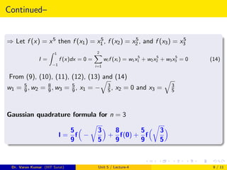
♦ Gauss quadrature 3-point formula ⇒ I = 5
9
f
−
q
3
5
+ 8
9
f (0) + 5
9
f
q
3
5
Interval Transformation:
⇒ Objective→ To find
R b
a f (x)dx
⇒ Interval transformation refers →
R b
a ⇐⇒
R 1
−1 and f (x) ⇐⇒ f (z)
Let
x = Az + B
dx = Adz
When I =
R b
a
f (x)dx =
R 1
−1
Af (z)dz = A
Pn
i=1 wi f (zi )
At x = a → z = −1 and x = b → z = 1
a = −A + B and b = A + B
A = b−a
2 and B = a+b
2
Dr. Varun Kumar (IIIT Surat) Unit 5 / Lecture-4 10 / 11

11. Continued–
For Gauss 2-point formula
I =
Z b
a
f (x)dx = A
2
X
i=1
wi f (zi ) =
b − a
2
[w1f (z1) + w2f (z2)] (15)
where w1 = w2 = 1 and z1 = − 1
√
3
, z2 = 1
√
3
For Gauss 3-point formula
I =
Z b
a
f (x)dx = A
3
X
i=1
wi f (zi ) =
b − a
2
[w1f (z1) + w2f (z2) + w3f (z3)]
(16)
where w1 = 5
9, w2 = 8
9, w3 = 5
9 and z1 = −
q
3
5, z2 = 0, z3 =
q
3
5
Dr. Varun Kumar (IIIT Surat) Unit 5 / Lecture-4 11 / 11