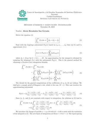
This document derives the Simpson's rule for numerical integration. It starts with the Lagrange polynomial used to approximate the integrand f(x). Replacing f(x) with the polynomial leads to an approximation of the integral as a weighted sum of the function values. For Simpson's rule with three equally spaced points x0, x1, x2, the approximating polynomial is given. Integrating this polynomial results in the Simpson's rule formula: the integral of f(x) from x0 to x2 is approximately equal to h/3(f0 + 4f1 + f2), where h is the spacing between points and fk = f(xk).

1. Centro de Investigaci´on y de Estudios Avanzados del Instituto Polit´ecnico
Nacional
Unidad Guadalajara
Sistemas el´ectricos de Potencia
M´etodos n´umericos y computaci´on: Investigaci´on
November 25, 2019
Nombre: Alexis Hern´andez San Germ´an
Derive the equation (1)
x2
x0
f(x)dx ≈
h
3
(f0 + 4f1 + f2) (1)
Start with the Lagrange polynomial PM (x) based on x0, x1, . . . , xM that can be used to
approximate f(x):
f(x) ≈ PM (x) =
M
k=0
fk LM,k(x) (2)
where fk = f(xk) for k = 0, 1, . . . , M. An approximation for the integral is obtained by
replacing the integrand f(x) with the polynomial PM (x). This is the general method for
obtaining a Newton-Cotes integration formula:
xM
x0
f(x)dx ≈
xM
x0
PM (x)dx
=
xM
x0
M
k=0
fk LM,k(x) dx =
M
k=0
xM
x0
fkLM,k(x)dx
=
M
k=0
xM
x0
LM,k(x)dx fk =
M
k=0
wkfk
(3)
The details for the general computations of the coefficients of wk in (3) are tedious. We
shall give a sample proof of Simpson’s rule, which is the case M = 2. This case involves the
approximating polynomial
P2(x) = f0
(x − x1)(x − x2)
(x0 − x1)(x0 − x2)
+ f1
(x − x0)(x − x2)
(x1 − x0)(x1 − x2)
+ f2
(x − x0)(x − x1)
(x2 − x0)(x2 − x1)
(4)
Since f0, f1, and f2 are constants with respect to integration, the relations in (3) lead to
x2
x0
f(x)dx ≈ f0
x2
x0
(x − x1)(x − x2)
(x0 − x1)(x0 − x2)
dx + f1
x2
x0
(x − x0)(x − x2)
(x1 − x0)(x1 − x2)
dx
+ f2
x2
x0
(x − x0)(x − x1)
(x2 − x0)(x2 − x1)
dx
(5)
We introduce the change of variable x = x0+ht with dx = h dt to assist with the evaluation
of the integrals in (5). The new limits of integration are from t = 0 to t = 2. The equal spacing
1

2. nodes xk = x0 + kh leads to xk − xj = (k − j)h and x − xk = h(t − k), which are used to
simplify (5) and get
x2
x0
f(x)dx ≈ f0
2
0
h(t − 1)h(t − 2)
(−h)(−2h)
h dt + f1
2
0
h(t − 0)h(t − 2)
(h)(−h)
h dt
+ f2
2
0
h(t − 0)h(t − 1)
(2h)(h)
h dt
= f0
h
2
2
0
(t2
− 3t + 2) dt − f1h
2
0
(t2
− 2t) dt + f2
h
2
2
0
(t2
− t) dt
= f0
h
2
t3
3
−
3t2
2
+ 2t
t=2
t=0
− f1h
t3
3
− t2
t=2
t=0
+ f2
h
2
t3
3
−
t2
2
t=2
t=0
= f0
h
2
2
3
− f1h
−4
3
+ f2
h
2
2
3
=
h
3
(f0 + 4f1 + f2)
(6)
References
[1] John H. Matthews, Kurtis K. Fink, Numerical Methods using MATLAB 4th Edition,
Pearson Education, 2010
2