The document discusses the paired t-test, which compares the means of two populations that are paired or matched. It explains that the paired t-test creates a new variable D that is the difference between each pair's x1 and x2 values. This D variable is then tested to see if its mean is significantly different from zero. The paired t-test has higher power than an independent t-test because individual differences are not part of the error term when comparing differences within each pair. However, it has limitations for some experimental designs where substantial time passes between measurements.

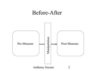
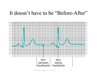
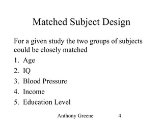
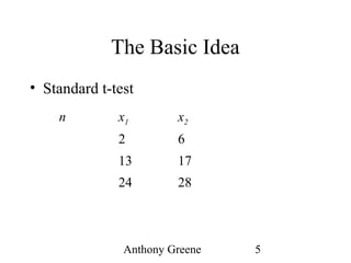
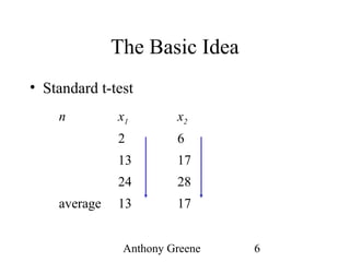
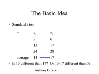
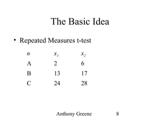
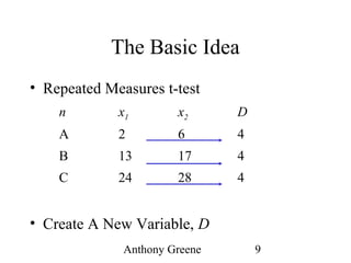
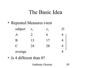
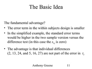
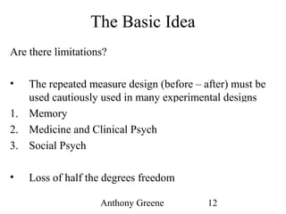
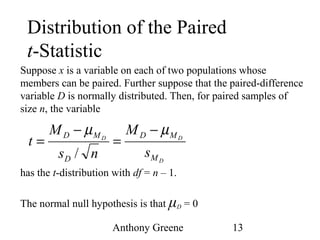
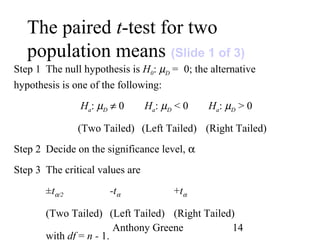
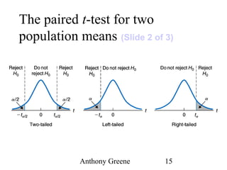
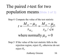
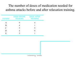
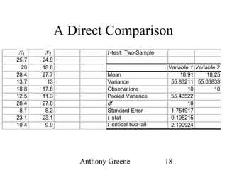
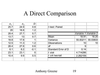
1. Paired t-test: tD
I. Introduction To The Repeated
Measures Design:What is a
repeated measure?
II. Finding an Experimental Effect In
a Single Group: Before vs. After
III. Creating a new distribution tD.
IV. Reduces Sampling Error: It’s a
more powerful test
V. Limited Applicability

2. Anthony Greene 2
Before-After
Pre-Measure Post-Measure
Manipulation

3. Anthony Greene 3
It doesn’t have to be “Before-After”

4. Anthony Greene 4
Matched Subject Design
For a given study the two groups of subjects
could be closely matched
1. Age
2. IQ
3. Blood Pressure
4. Income
5. Education Level

5. Anthony Greene 5
The Basic Idea
• Standard t-test
n x1 x2
2 6
13 17
24 28

6. Anthony Greene 6
The Basic Idea
• Standard t-test
n x1 x2
2 6
13 17
24 28
average 13 17

7. Anthony Greene 7
The Basic Idea
• Standard t-test
• Is 13 different than 17? Or 13-17 different than 0?
n x1 x2
2 6
13 17
24 28
average 13 17

8. Anthony Greene 8
The Basic Idea
• Repeated Measures t-test
n x1 x2
A 2 6
B 13 17
C 24 28

9. Anthony Greene 9
The Basic Idea
• Repeated Measures t-test
• Create A New Variable, D
n x1 x2 D
A 2 6 4
B 13 17 4
C 24 28 4

10. Anthony Greene 10
The Basic Idea
• Repeated Measures t-test
• Is 4 different than 0?
subject x1 x2 D
A 2 6 4
B 13 17 4
C 24 28 4
average 4

11. Anthony Greene 11
The Basic Idea
The fundamental advantage?
• The error term in the within subjects design is smaller
• In the simplified example, the standard error terms
would be higher in the two sample version versus the
difference test (in this case the sMD
is zero)
• The advantage is that individual differences
(2, 13, 24, and 5, 16, 27) are not part of the error in tD

12. Anthony Greene 12
The Basic Idea
Are there limitations?
• The repeated measure design (before – after) must be
used cautiously used in many experimental designs
1. Memory Subjects learn
2. Medicine and Clinical Psych Substantial time passes
3. Social Psych Minor deceptions
• Loss of half the degrees freedom

13. Anthony Greene 13
Distribution of the Paired
t-Statistic
Suppose x is a variable on each of two populations whose
members can be paired. Further suppose that the paired-difference
variable D is normally distributed. Then, for paired samples of
size n, the variable
has the t-distribution with df = n – 1.
The normal null hypothesis is that μD = 0
D
DD
M
MD
D
MD
s
M
ns
M
t
µµ −
=
−
=
/

14. Anthony Greene 14
The paired t-test for two
population means (Slide 1 of 3)
Step 1 The null hypothesis is H0: µD = 0; the alternative
hypothesis is one of the following:
Ha: µD ≠ 0 Ha: µD < 0 Ha: µD > 0
(Two Tailed) (Left Tailed) (Right Tailed)
Step 2 Decide on the significance level, α
Step 3 The critical values are
±tα/2 -tα +tα
(Two Tailed) (Left Tailed) (Right Tailed)
with df = n - 1.

15. Anthony Greene 15
The paired t-test for two
population means (Slide 2 of 3)

16. Anthony Greene 16
The paired t-test for two
population means(Slide 3 of 3)
Step 4 Compute the value of the test statistic
Step 5 If the value of the test statistic falls in the
rejection region, reject H0, otherwise do not
reject H0.
0normallywhere
/
=
−
=
−
=
D
D
DD
M
DD
ns
M
s
M
t
D
µ
µµ

17. Anthony Greene 17
The number of doses of medication needed for
asthma attacks before and after relaxation training.
72.3
592.1
2.3
92.1
4
8.14
1
−=
−
==
==
−
=
DM
D
D
s
M
t
n
SS
s

18. Anthony Greene 18
A Direct Comparison
x1 x2 t -test: Two-Sample
25.7 24.9
20 18.8 Variable 1 Variable 2
28.4 27.7 Mean 18.91 18.25
13.7 13 Variance 55.83211 55.03833
18.8 17.8 Observations 10 10
12.5 11.3 Pooled Variance 55.43522
28.4 27.8 df 18
8.1 8.2 Standard Error 1.754917
23.1 23.1 t stat 0.198215
10.4 9.9 t critical two-tail 2.100924
x1 x2

19. Anthony Greene 19
A Direct Comparison
x1 x2 D
25.7 24.9 0.8 t -test: Paired
20 18.8 1.2
28.4 27.7 0.7 Variable 1 Variable 2
13.7 13 0.7 Mean 18.91 18.25
18.8 17.8 1 Variance 55.83211 55.03833
12.5 11.3 1.2 Observations 10 10
28.4 27.8 0.6 df 9
8.1 8.2 -0.1 Standard Error of D 0.14
23.1 23.1 0 t stat 4.714286
10.4 9.9 0.5 t crit two-tail 2.262159
x1 x2