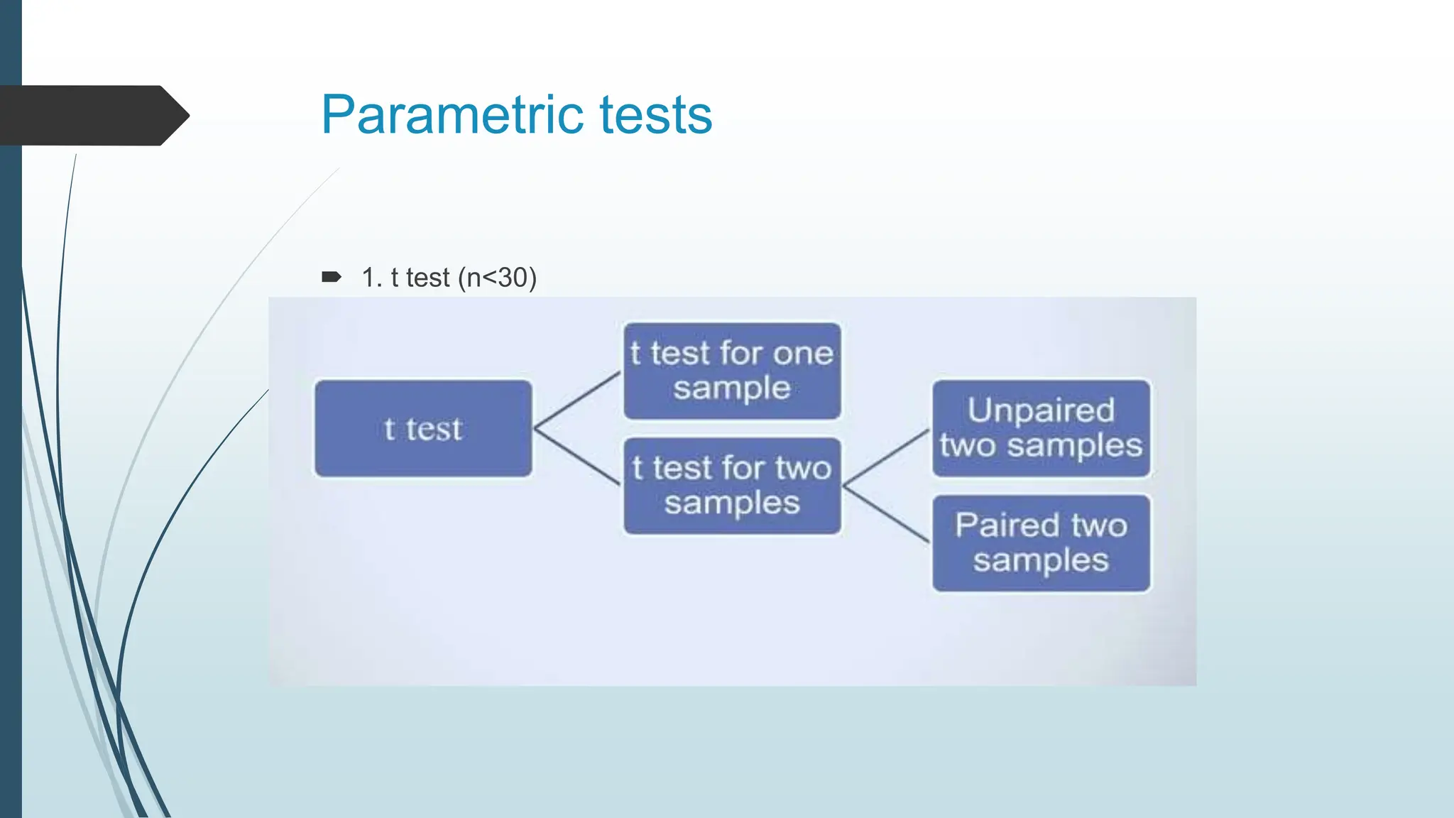
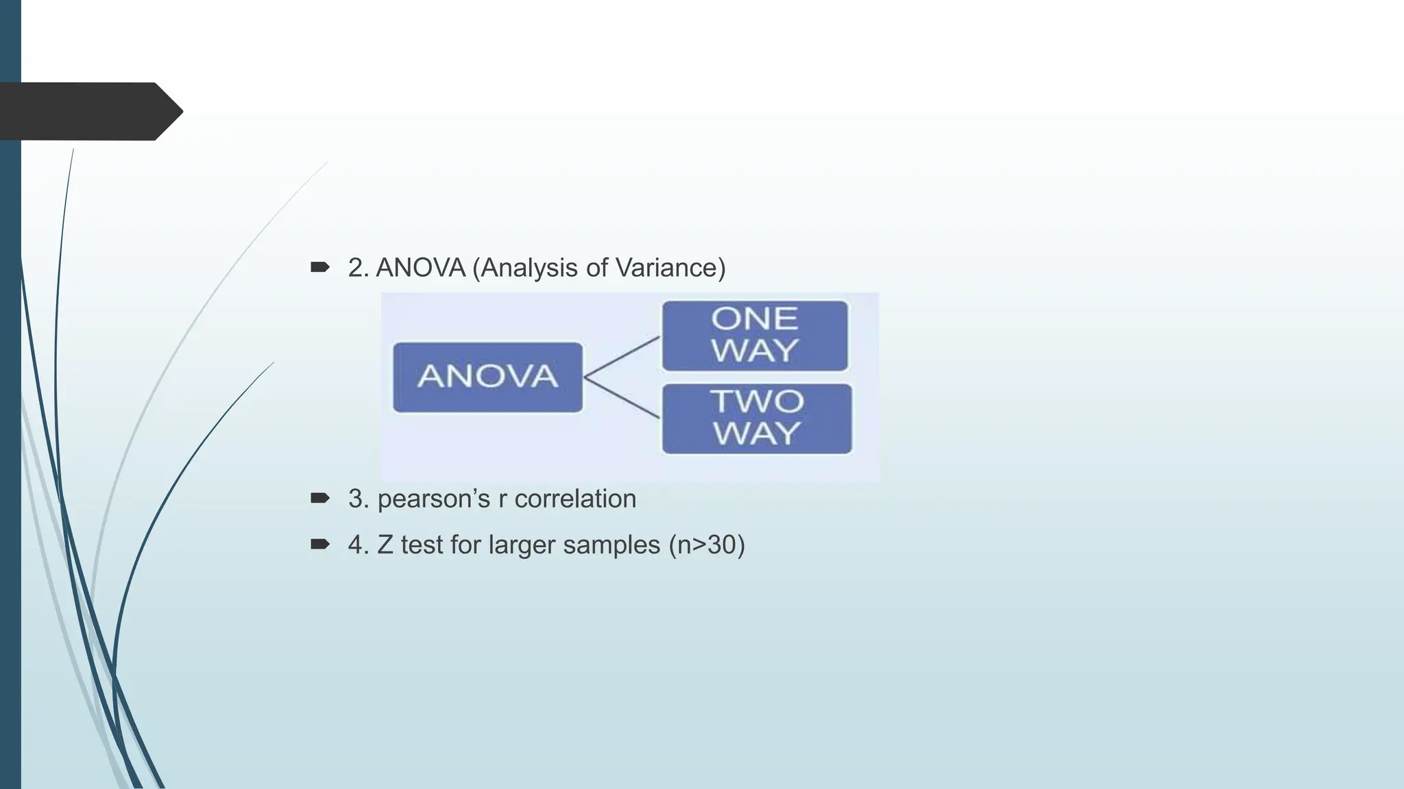
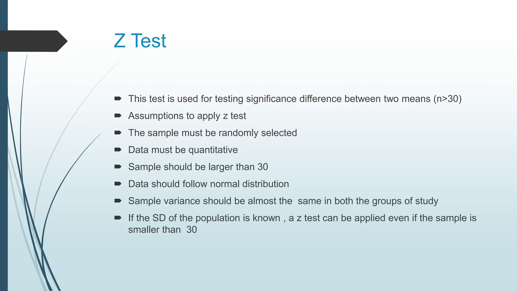
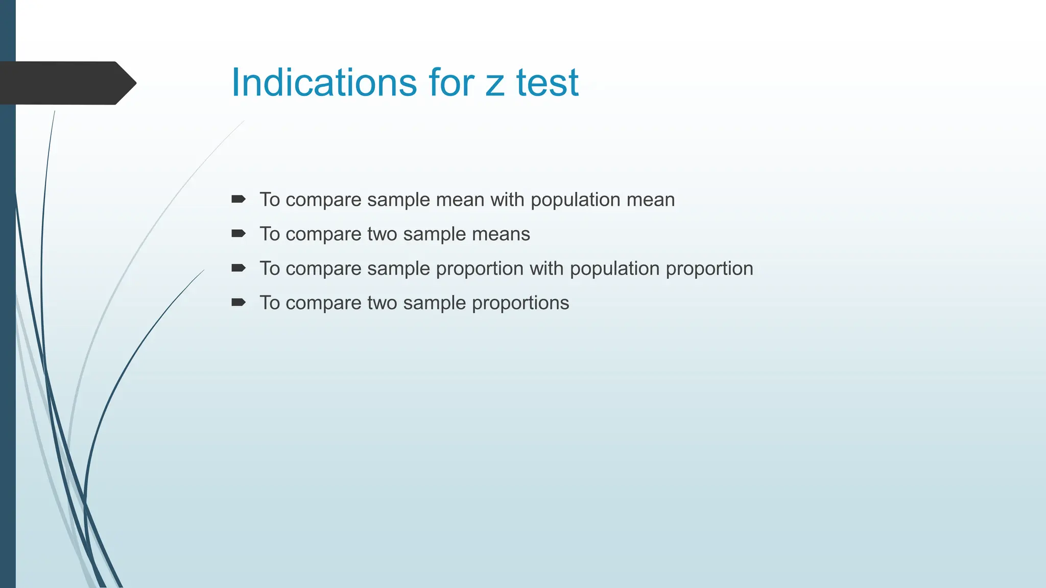
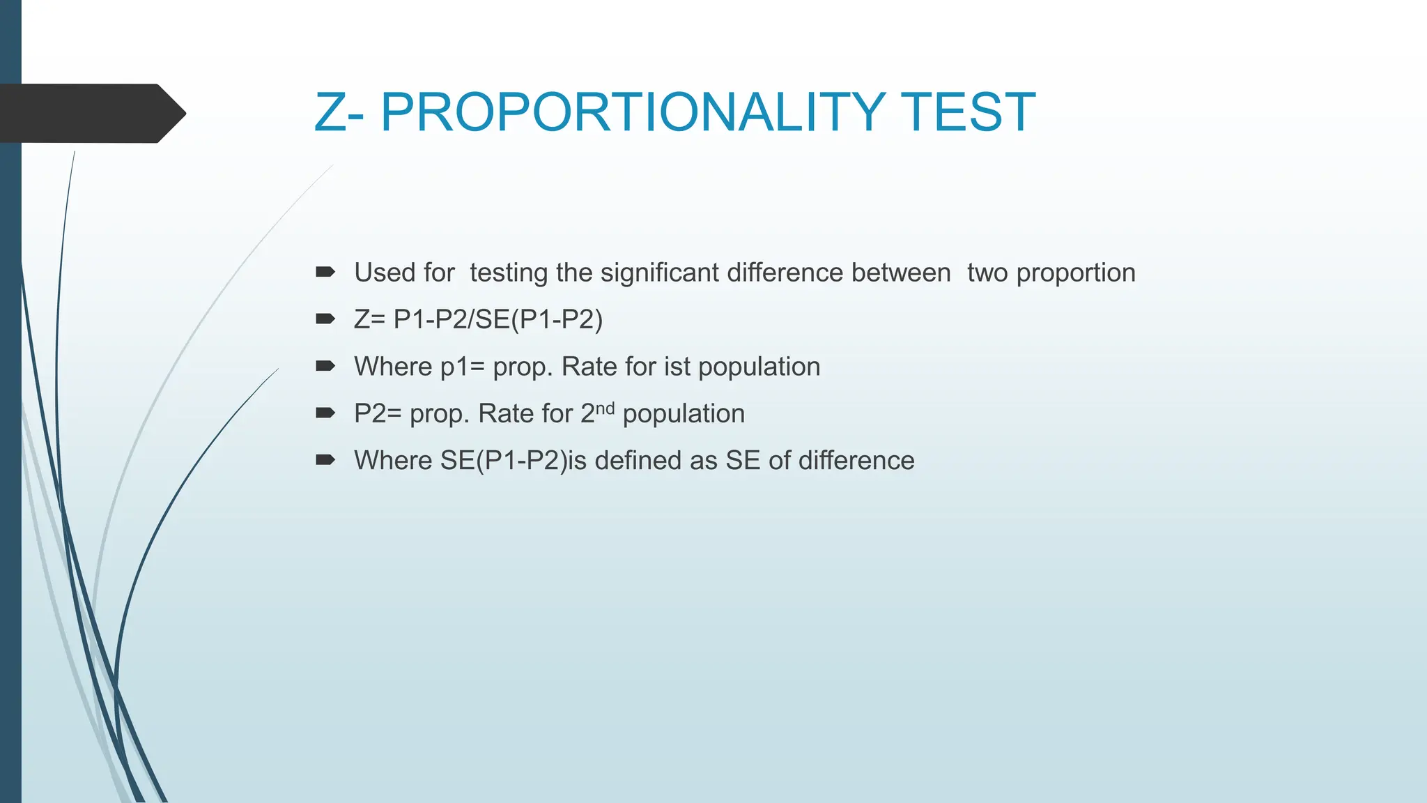
PARAMETRIC TESTS
Dr. Aastha Sahani
Dr. Dimple Chawla
Dr. Mahima Jain
Dr. Sauhard Sachdeva
Dr. Pallavi Kumari
Dr. Sonal Aggarwal
CONTENTS
 Introduction to statistical tests
 System for statistical analysis
 Parametric tests
 t test
 ANOVA
 Pearson’s coefficient of correlation
 Z test
 Conclusion
 References
Statistical Test
 These are intended to decide whether a hypothesis about distribution of one or
more populations should be rejected or accepted
 These may be
 These tests the statistical significance of the:
1) Difference in sample and population mean
2) Difference in two sample means
3) Several population means
4) Difference in proportions between sample and population
5) Difference in proportions between two independent populations
6) Significance of association between two variables
SYSTEM FOR STATISTICAL ANALYSIS
 State the research hypothesis
 State the level of significance
 Calculate the test statistic
 Compare the calculated test statistic with the tabulated values
 Decision
 Statement of result
Parametric Tests
 Used for quantitative data
 Used for continuous variables
 Used when data is measured on approximate interval or ratio scales of
measurement
 Data should follow normal distribution
Parametric tests
 1. t test (n<30)
 2. ANOVA (Analysis of Variance)
 3. pearson’s r correlation
 4. Z test for larger samples (n>30)
One tailed and two tailed tests
 Z values on each side of mean are calculated as +z or –z
 A result larger than difference between sample will give +z and result smaller than
differnce between mean will give –z
 Eg for two tailed :
 In a test of significance , when one wants to determine whether the mean iq of
malnourished children is different from that of well nourished and soes not specify
higher or lower , the p value of an experiment group includes both sides of extreme
result at both ends of scale , and the test is called two tailed test
STUDENT’S T TEST
 Developed by Prof W.S. Gossett in 1908, who published statistical papers
under the pen name of ‘Student’. Thus the test is known as Student’s ‘t’
test.
 Indiacations for the test:
1. When samples are small
2. Population variance are not known.
USES
 Two means of small independent samples
 Sample mean and population mean
 Two proportions of small independent samples
ASSUMPTIONS MADE IN THE USE OF
‘T’ TEST
 Samples are randomly selected.
 Data utilized is quantitative.
 Variable follow normal distribution.
 Sample variances are mostly same in both the groups under the study.
 Samples are small, mostly lower than 30.
 A t-test compares the difference between two means of different groups to
determine whether that difference is statistically significant.
 Student’s ‘t’ test for different purposes
• ‘t’ test for one sample
• ‘t’ test for unpaired two samples
• ‘t’ test for paired two samples
ONE SAMPLE T-TEST
 When compare the mean of single group of observations with a specified
value
 In one sample t test, we know the population mean.
 We draw a random sample from the population and then compare the
sample mean with the population mean and make a statistical decision as
to whether or not the sample mean is different from the population.
CALCULATION
 Now we compare calculated value with table value at certain level of
significance (generally 5% or 1%)
 If absolute value of ‘t’ obtained is greater is greater than table value then
reject the null hypothesis and if it is less than table value, the null
hypothesis may be accepted.
EXAMPLE
 Research problem: comparison of mean dietary intake of a particular group of
individuals with the recommended daily intake.
 DATA: Average daily energy intake (ADEI) over 10 days of 11 healthy women
 Mean ADEI value = 6753.6
 SD ADEI value = 1142.1
 When can we say about the energy intake of these women in relation to a
recommended daily intake of 7725 KL?
sub 1 2 3 4 5 6 7 8 9 10 11
ADEI 5260 5470 5640 6180 6390 6515 6805 7515 7515 8230 8770
RESEARCH HYPOTHESIS
 State null hypothesis and alternative hypothesis:
H0 = there is no difference between population mean and sample mean
OR
H0: µ = 7725 KJ
H1 = there is a difference between population mean and sample mean
OR
H1 : µ ≠ 7725 KJ
 Set the level of significance
 α = .05, .01 or .001
 Calculate the value of proper statistic
 T = sample mean – hypothesized mean/standard error of sample mean
 6753.6 – 7725 ÷ 1142.1/ √11 = -0.2564
State the rule for rejecting the null
hypothesis
 In the above example we have seen t = -.2564 which is less than 2.23
 P value suggest that the dietary intake of these women was significantly less than
recommended level (7725 KJ)
Two Sample ‘t’ test
A. Unpaired Two sample ‘t’ test
Unpaired t-test is used when we wish to compare two means.
Used when the two independent random samples come from the
normal populations having unknown or same variance.
We test the null hypothesis, that the two population means are
same i.e µ1=µ2 against an appropriate one sided alternative hypothesis.
Assumptions
The samples are random and independent of each
other
The distribution of dependant variable is normal
The variances are equal in both the groups
FORMULA
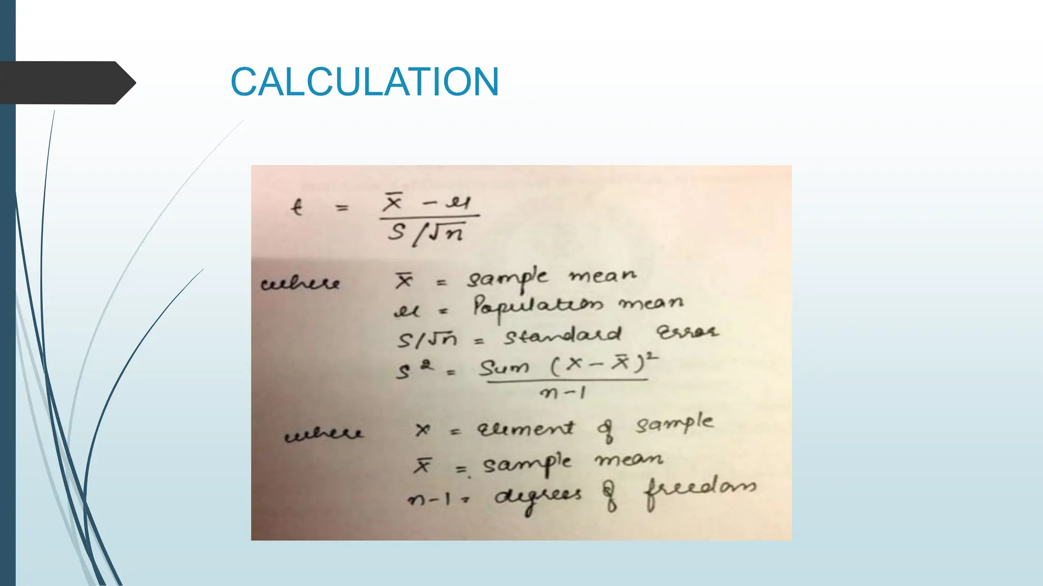
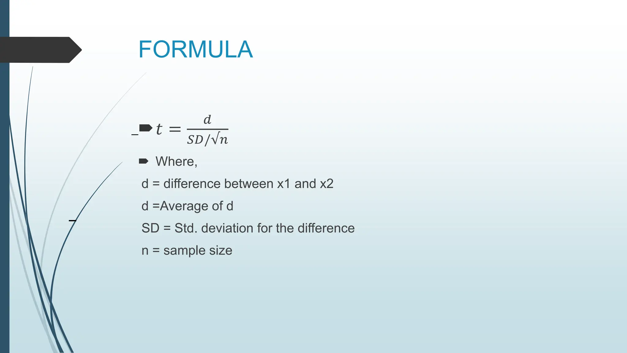
Test statistics is given by
t= Mean 1- Mean2
SE(Mean1- Mean2)
SE(Mean1 – Mean2) = s [1/n1 + 1/n2]
S= (n1 – 1)S12
w
2
1
2
1
1
1
n
n
s
x
x
test
t



RESEARCH PROBLEM
A study was conducted to compare the birth weights of children
born to 15 non-smoking with those of children born to 14 heavy
smoking mothers.
Research Hypothesis : state null hypothesis and
alternative hypothesis
Ho there is no difference between the birth weights of
children born to non-smoking and smoking mothers
H1 = there is a difference between the birth weights of
children born to non-smoking and smoking mothers
Set the level of significance
α = .05, .01 or .001
Calculate the value of proper statistic
State the rule for rejecting the null hypothesis
If tcal > ttab we can say that P< .05 then we reject the
null hypothesis and accept the alternative hypothesis
decision
if we reject the null hypothesis so we can say that
children born to non-smokers are heavier than
children born to heavy smokers.
Paired Two Samples T-test
 Used when we have paired data of observations from one sample only,
when each individual gives a pair of observations.
 Same individuals are studied more than once in different circumstances-
measurements made on the same people before and after interventions.
Assumptions
 The outcome variable should be continuous.
 The difference between pre-post measurements should be normally
distributed.
FORMULA
𝑡 =
𝑑
𝑆𝐷/√𝑛
 Where,
d = difference between x1 and x2
d =Average of d
SD = Std. deviation for the difference
n = sample size
¯
¯
Research Problem
 A study was carried to evaluate the effect of the new diet on weight loss.
The study population consist of 12 people have used the diet for 2 months;
their weights before and after the diet are given.
Patient no. Weight (kgs)
Before Diet After Diet
1 75 70
2 60 54
3 68 58
4 98 93
5 83 78
6 89 84
7 65 60
8 78 77
9 95 90
10 80 76
11 100 94
12 108 100
Research Hypothesis
 State null hypothesis and alternative hypothesis
 H0 = There is no reduction in weight after Diet
 H1=There is reduction in weight after Diet
 Further Analysis through Statistical software SPSS as same as previous
example.
Decision
 If we reject the null hypothesis then there is a statistically significant
reduction in weight.
How do we compare more than two groups
means ?
 Example:
 Treatments: A, B, C &D
 Response: BP level
 How does t-test concept work here?
A versus B B versus C
A versus C B versus D
A versus D C versus D
 so the chance of getting the wrong result would be:
1 - (0.95 x 0.95 x 0.95 x0.95) = 26%
 Instead of using a series of individual comparisons we examine the
differences among the groups through an analysis that considers the
variation among all groups at once.
 i.e. ANALYSIS OF VARIANCE.
Analysis of Variance (ANOVA)
 Given by Sir Ronald Fisher
 The principle aim of statistical models is to explain the variation in measurements
 The statistical model involving a test of significance of the difference in mean
values of the variable between 2 groups is the student’s t test. If there are more
than 2 groups, the statistical model is ANOVA
Assumptions for ANOVA
 Sample population can be easily approximated to normal distribution
 All populations have same Standard Deviation
 Individuals in population are selected randomly
 Independent samples
 ANOVA compares variance by means of a simple ratio, called the F ratio
 The resulting F statistics is then compared with critical value of F (critic), obtained
from F tables in much same way as was done with the ‘t’
 If the calculated value exceeds the critical value for the appropriate level of α, the
null hypothesis will be rejected
 A F test is therefore a test of Ratio of Variances. F tests can also be used on their
own, independently of the ANOVA technique, to test hypothesis about variances
 In ANOVA, the F test is used to establish whether a statistically significant
difference exists in the data being tested
 ANOVA can be
 One way ANOVA
 if the various experimental groups differ in terms of only one factor at a time- a
one way ANOVA is used
Eg. A study to assess the effectiveness of four different antibiotics on S Sanguis
 Two Way ANOVA
 if the various groups differ in terms of two or more factors at a time, then a Two
Way ANOVA is performed
Eg. A study to assess the effectiveness of four different antibiotics on S Sanguis in
three different age groups
Pearson’s Correlation Coefficient
 Correlation is a technique for investigating the relationship between two
quantitative continuous variables
 Pearson’s Correlation Coefficient (r) is a measure of the strength of the association
between the two variables
Assumptions Made in Calculation of ‘r’
 Subjects selected for study with pair of values of X&Y are chosen with random
sampling procedure
 Both X & Y variables are continuous
 Both variables X & Y are assumed to follow normal distribution
Steps
 The first step in studying the relatioship between two continuous variables is to
draw a scatter plot of the variables to check for linearity
 The correlation coefficient should not be calculated of the relationships is not linear
 For correlation only purposes ,it does not matter on which axis the variables are
plotted
 However ,conventionally the independent variable is plottedon X axis and
dependent variable on Y axis
 The nearer the scatter of points is to a straight line,the higher the strength of
association between variables
Types of Correlation
 Perfect positive correlation r=+1
 Partial positive correlation 0<r<+1
 Perfect negative correlation r =-1
 Partial negative correlation 0>r>1
 No correlation
Z Test
 This test is used for testing significance difference between two means (n>30)
 Assumptions to apply z test
 The sample must be randomly selected
 Data must be quantitative
 Sample should be larger than 30
 Data should follow normal distribution
 Sample variance should be almost the same in both the groups of study
 If the SD of the population is known , a z test can be applied even if the sample is
smaller than 30
Indications for z test
 To compare sample mean with population mean
 To compare two sample means
 To compare sample proportion with population proportion
 To compare two sample proportions
steps
 Define the problem
 State the null hypothesis (HO)and alternate hypothesis
 Find z value
 Z= OBSERVED MEAN – MEAN /STANDARD ERROR
 Fix the level of significance
 Compare calculated z value with the value in the z table at corresponding degree
significance level
 If the observed Z value is greater than theoritical Z value , Z is significant , reject
null hypothesis and accept alternate hypothesis
Z- PROPORTIONALITY TEST
 Used for testing the significant difference between two proportion
 Z= P1-P2/SE(P1-P2)
 Where p1= prop. Rate for ist population
 P2= prop. Rate for 2nd population
 Where SE(P1-P2)is defined as SE of difference
THANK YOU

Epidemiological study design and it's significance

  • 1.
    PARAMETRIC TESTS Dr. AasthaSahani Dr. Dimple Chawla Dr. Mahima Jain Dr. Sauhard Sachdeva Dr. Pallavi Kumari Dr. Sonal Aggarwal
  • 2.
    CONTENTS  Introduction tostatistical tests  System for statistical analysis  Parametric tests  t test  ANOVA  Pearson’s coefficient of correlation  Z test  Conclusion  References
  • 3.
    Statistical Test  Theseare intended to decide whether a hypothesis about distribution of one or more populations should be rejected or accepted  These may be
  • 4.
     These teststhe statistical significance of the: 1) Difference in sample and population mean 2) Difference in two sample means 3) Several population means 4) Difference in proportions between sample and population 5) Difference in proportions between two independent populations 6) Significance of association between two variables
  • 5.
    SYSTEM FOR STATISTICALANALYSIS  State the research hypothesis  State the level of significance  Calculate the test statistic  Compare the calculated test statistic with the tabulated values  Decision  Statement of result
  • 6.
    Parametric Tests  Usedfor quantitative data  Used for continuous variables  Used when data is measured on approximate interval or ratio scales of measurement  Data should follow normal distribution
  • 7.
  • 8.
     2. ANOVA(Analysis of Variance)  3. pearson’s r correlation  4. Z test for larger samples (n>30)
  • 11.
    One tailed andtwo tailed tests  Z values on each side of mean are calculated as +z or –z  A result larger than difference between sample will give +z and result smaller than differnce between mean will give –z
  • 12.
     Eg fortwo tailed :  In a test of significance , when one wants to determine whether the mean iq of malnourished children is different from that of well nourished and soes not specify higher or lower , the p value of an experiment group includes both sides of extreme result at both ends of scale , and the test is called two tailed test
  • 13.
    STUDENT’S T TEST Developed by Prof W.S. Gossett in 1908, who published statistical papers under the pen name of ‘Student’. Thus the test is known as Student’s ‘t’ test.  Indiacations for the test: 1. When samples are small 2. Population variance are not known.
  • 14.
    USES  Two meansof small independent samples  Sample mean and population mean  Two proportions of small independent samples
  • 15.
    ASSUMPTIONS MADE INTHE USE OF ‘T’ TEST  Samples are randomly selected.  Data utilized is quantitative.  Variable follow normal distribution.  Sample variances are mostly same in both the groups under the study.  Samples are small, mostly lower than 30.
  • 16.
     A t-testcompares the difference between two means of different groups to determine whether that difference is statistically significant.  Student’s ‘t’ test for different purposes • ‘t’ test for one sample • ‘t’ test for unpaired two samples • ‘t’ test for paired two samples
  • 17.
    ONE SAMPLE T-TEST When compare the mean of single group of observations with a specified value  In one sample t test, we know the population mean.  We draw a random sample from the population and then compare the sample mean with the population mean and make a statistical decision as to whether or not the sample mean is different from the population.
  • 18.
  • 19.
     Now wecompare calculated value with table value at certain level of significance (generally 5% or 1%)  If absolute value of ‘t’ obtained is greater is greater than table value then reject the null hypothesis and if it is less than table value, the null hypothesis may be accepted.
  • 20.
    EXAMPLE  Research problem:comparison of mean dietary intake of a particular group of individuals with the recommended daily intake.  DATA: Average daily energy intake (ADEI) over 10 days of 11 healthy women  Mean ADEI value = 6753.6  SD ADEI value = 1142.1  When can we say about the energy intake of these women in relation to a recommended daily intake of 7725 KL? sub 1 2 3 4 5 6 7 8 9 10 11 ADEI 5260 5470 5640 6180 6390 6515 6805 7515 7515 8230 8770
  • 21.
    RESEARCH HYPOTHESIS  Statenull hypothesis and alternative hypothesis: H0 = there is no difference between population mean and sample mean OR H0: µ = 7725 KJ H1 = there is a difference between population mean and sample mean OR H1 : µ ≠ 7725 KJ
  • 22.
     Set thelevel of significance  α = .05, .01 or .001  Calculate the value of proper statistic  T = sample mean – hypothesized mean/standard error of sample mean  6753.6 – 7725 ÷ 1142.1/ √11 = -0.2564
  • 23.
    State the rulefor rejecting the null hypothesis  In the above example we have seen t = -.2564 which is less than 2.23  P value suggest that the dietary intake of these women was significantly less than recommended level (7725 KJ)
  • 24.
    Two Sample ‘t’test A. Unpaired Two sample ‘t’ test Unpaired t-test is used when we wish to compare two means. Used when the two independent random samples come from the normal populations having unknown or same variance. We test the null hypothesis, that the two population means are same i.e µ1=µ2 against an appropriate one sided alternative hypothesis.
  • 25.
    Assumptions The samples arerandom and independent of each other The distribution of dependant variable is normal The variances are equal in both the groups
  • 26.
    FORMULA Test statistics isgiven by t= Mean 1- Mean2 SE(Mean1- Mean2) SE(Mean1 – Mean2) = s [1/n1 + 1/n2] S= (n1 – 1)S12 w 2 1 2 1 1 1 n n s x x test t   
  • 27.
    RESEARCH PROBLEM A studywas conducted to compare the birth weights of children born to 15 non-smoking with those of children born to 14 heavy smoking mothers.
  • 29.
    Research Hypothesis :state null hypothesis and alternative hypothesis Ho there is no difference between the birth weights of children born to non-smoking and smoking mothers H1 = there is a difference between the birth weights of children born to non-smoking and smoking mothers Set the level of significance α = .05, .01 or .001
  • 30.
    Calculate the valueof proper statistic State the rule for rejecting the null hypothesis If tcal > ttab we can say that P< .05 then we reject the null hypothesis and accept the alternative hypothesis decision if we reject the null hypothesis so we can say that children born to non-smokers are heavier than children born to heavy smokers.
  • 31.
    Paired Two SamplesT-test  Used when we have paired data of observations from one sample only, when each individual gives a pair of observations.  Same individuals are studied more than once in different circumstances- measurements made on the same people before and after interventions.
  • 32.
    Assumptions  The outcomevariable should be continuous.  The difference between pre-post measurements should be normally distributed.
  • 33.
    FORMULA 𝑡 = 𝑑 𝑆𝐷/√𝑛  Where, d= difference between x1 and x2 d =Average of d SD = Std. deviation for the difference n = sample size ¯ ¯
  • 34.
    Research Problem  Astudy was carried to evaluate the effect of the new diet on weight loss. The study population consist of 12 people have used the diet for 2 months; their weights before and after the diet are given.
  • 35.
    Patient no. Weight(kgs) Before Diet After Diet 1 75 70 2 60 54 3 68 58 4 98 93 5 83 78 6 89 84 7 65 60 8 78 77 9 95 90 10 80 76 11 100 94 12 108 100
  • 36.
    Research Hypothesis  Statenull hypothesis and alternative hypothesis  H0 = There is no reduction in weight after Diet  H1=There is reduction in weight after Diet  Further Analysis through Statistical software SPSS as same as previous example. Decision  If we reject the null hypothesis then there is a statistically significant reduction in weight.
  • 37.
    How do wecompare more than two groups means ?  Example:  Treatments: A, B, C &D  Response: BP level  How does t-test concept work here? A versus B B versus C A versus C B versus D A versus D C versus D  so the chance of getting the wrong result would be: 1 - (0.95 x 0.95 x 0.95 x0.95) = 26%
  • 38.
     Instead ofusing a series of individual comparisons we examine the differences among the groups through an analysis that considers the variation among all groups at once.  i.e. ANALYSIS OF VARIANCE.
  • 39.
    Analysis of Variance(ANOVA)  Given by Sir Ronald Fisher  The principle aim of statistical models is to explain the variation in measurements  The statistical model involving a test of significance of the difference in mean values of the variable between 2 groups is the student’s t test. If there are more than 2 groups, the statistical model is ANOVA
  • 40.
    Assumptions for ANOVA Sample population can be easily approximated to normal distribution  All populations have same Standard Deviation  Individuals in population are selected randomly  Independent samples
  • 41.
     ANOVA comparesvariance by means of a simple ratio, called the F ratio  The resulting F statistics is then compared with critical value of F (critic), obtained from F tables in much same way as was done with the ‘t’  If the calculated value exceeds the critical value for the appropriate level of α, the null hypothesis will be rejected
  • 42.
     A Ftest is therefore a test of Ratio of Variances. F tests can also be used on their own, independently of the ANOVA technique, to test hypothesis about variances  In ANOVA, the F test is used to establish whether a statistically significant difference exists in the data being tested  ANOVA can be
  • 43.
     One wayANOVA  if the various experimental groups differ in terms of only one factor at a time- a one way ANOVA is used Eg. A study to assess the effectiveness of four different antibiotics on S Sanguis
  • 44.
     Two WayANOVA  if the various groups differ in terms of two or more factors at a time, then a Two Way ANOVA is performed Eg. A study to assess the effectiveness of four different antibiotics on S Sanguis in three different age groups
  • 45.
    Pearson’s Correlation Coefficient Correlation is a technique for investigating the relationship between two quantitative continuous variables  Pearson’s Correlation Coefficient (r) is a measure of the strength of the association between the two variables
  • 46.
    Assumptions Made inCalculation of ‘r’  Subjects selected for study with pair of values of X&Y are chosen with random sampling procedure  Both X & Y variables are continuous  Both variables X & Y are assumed to follow normal distribution
  • 47.
    Steps  The firststep in studying the relatioship between two continuous variables is to draw a scatter plot of the variables to check for linearity  The correlation coefficient should not be calculated of the relationships is not linear  For correlation only purposes ,it does not matter on which axis the variables are plotted
  • 48.
     However ,conventionallythe independent variable is plottedon X axis and dependent variable on Y axis  The nearer the scatter of points is to a straight line,the higher the strength of association between variables
  • 49.
    Types of Correlation Perfect positive correlation r=+1  Partial positive correlation 0<r<+1  Perfect negative correlation r =-1  Partial negative correlation 0>r>1  No correlation
  • 50.
    Z Test  Thistest is used for testing significance difference between two means (n>30)  Assumptions to apply z test  The sample must be randomly selected  Data must be quantitative  Sample should be larger than 30  Data should follow normal distribution  Sample variance should be almost the same in both the groups of study  If the SD of the population is known , a z test can be applied even if the sample is smaller than 30
  • 51.
    Indications for ztest  To compare sample mean with population mean  To compare two sample means  To compare sample proportion with population proportion  To compare two sample proportions
  • 52.
    steps  Define theproblem  State the null hypothesis (HO)and alternate hypothesis  Find z value  Z= OBSERVED MEAN – MEAN /STANDARD ERROR  Fix the level of significance  Compare calculated z value with the value in the z table at corresponding degree significance level  If the observed Z value is greater than theoritical Z value , Z is significant , reject null hypothesis and accept alternate hypothesis
  • 53.
    Z- PROPORTIONALITY TEST Used for testing the significant difference between two proportion  Z= P1-P2/SE(P1-P2)  Where p1= prop. Rate for ist population  P2= prop. Rate for 2nd population  Where SE(P1-P2)is defined as SE of difference
  • 54.