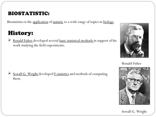
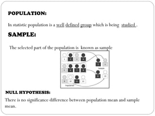
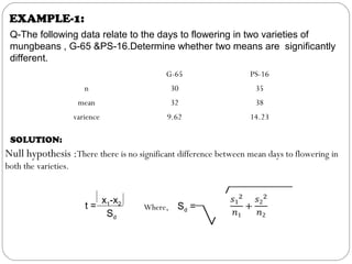
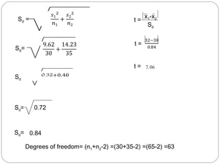
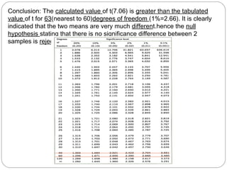
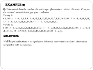
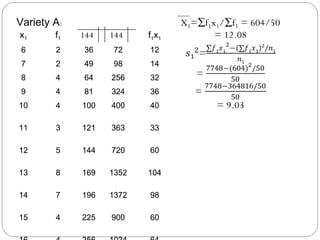
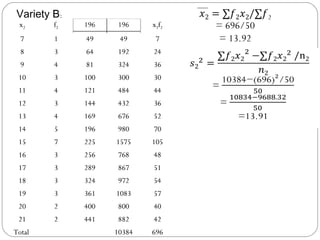
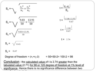
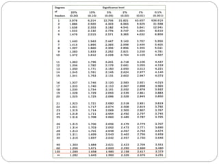
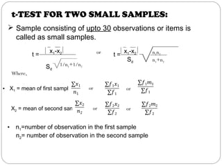
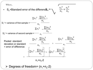
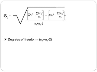
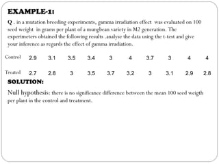
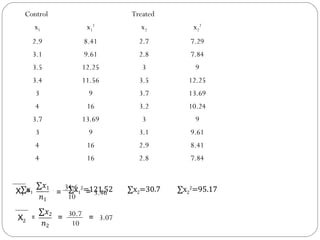
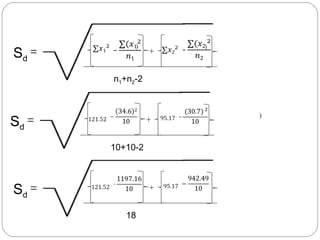
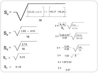
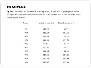
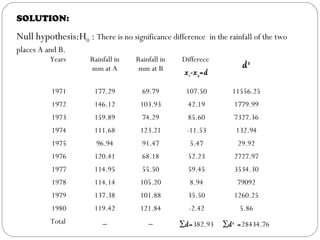
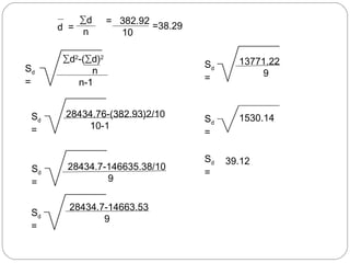
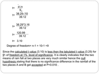
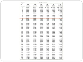
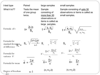
Today’s overwhelming number of techniques applicable to data analysis makes it extremely difficult to define the most beneficial approach while considering all the significant variables.
The analysis of variance has been studied from several approaches, the most common of which uses a linear model that relates the response to the treatments and blocks. Note that the model is linear in parameters but may be nonlinear across factor levels. Interpretation is easy when data is balanced across factors but much deeper understanding is needed for unbalanced data.
Analysis of variance (ANOVA) is a collection of statistical models and their associated estimation procedures (such as the "variation" among and between groups) used to analyze the differences among means. ANOVA was developed by the statistician Ronald Fisher. ANOVA is based on the law of total variance, where the observed variance in a particular variable is partitioned into components attributable to different sources of variation. In its simplest form, ANOVA provides a statistical test of whether two or more population means are equal, and therefore generalizes the t-test beyond two means. In other words, the ANOVA is used to test the difference between two or more means.Analysis of variance (ANOVA) is an analysis tool used in statistics that splits an observed aggregate variability found inside a data set into two parts: systematic factors and random factors. The systematic factors have a statistical influence on the given data set, while the random factors do not. Analysts use the ANOVA test to determine the influence that independent variables have on the dependent variable in a regression study.
Sir Ronald Fisher pioneered the development of ANOVA for analyzing results of agricultural experiments.1 Today, ANOVA is included in almost every statistical package, which makes it accessible to investigators in all experimental sciences. It is easy to input a data set and run a simple ANOVA, but it is challenging to choose the appropriate ANOVA for different experimental designs, to examine whether data adhere to the modeling assumptions, and to interpret the results correctly. The purpose of this report, together with the next 2 articles in the Statistical Primer for Cardiovascular Research series, is to enhance understanding of ANVOA and to promote its successful use in experimental cardiovascular research. My colleagues and I attempt to accomplish those goals through examples and explanation, while keeping within reason the burden of notation, technical jargon, and mathematical equations.
This presentation contains information about Mann Whitney U test, what is it, when to use it and how to use it. I have also put an example so that it may help you to easily understand it.
1 FACULTY OF SCIENCE AND ENGINEERING SCHOOL OF COMPUT.docxmercysuttle
1
FACULTY OF SCIENCE AND ENGINEERING
SCHOOL OF COMPUTING, MATHEMATICS & DIGITAL MEDIA
REASSESSMENT COURSEWORK 2013/14
UNIT CODE:
6G6Z3005
UNIT DESC:
APPLIED REGRESSION AND MULTIVARIATE ANALYSIS
ASSESSMENT ID:
1CWK30
ASSESSMENT NAME:
Courswork 30%
WEIGHT
FACTOR: 30%
See below.
NAME OF STAFF SETTING ASSIGNMENT: Dr B L Shea
0
MANCHESTER METROPOLITAN UNIVERSITY
FACULTY OF SCIENCE AND ENGINEERING
SCHOOL OF COMPUTING, MATHEMATICS & DIGITAL TECHNOLOGY
ACADEMIC YEAR 2013-2014:
REFERRED COURSEWORK
BSC(HONS) FINANCIAL MATHEMATICS
BSC(HONS) MATHEMATICS
YEAR/STAGE THREE
UNIT 6G6Z3005 : APPLIED REGRESSION AND MULTIVARIATE ANALYSIS
Answer ALL questions.
The pass mark is 40% which corresponds to a minimum of 72
marks out of a possible 180 marks.
The deadline is 8th August 2014.
SECTION A
1. (a) Three measurementsx1, x2 andx3 have the following sample covariance matrix.
∑̂ =
9 2 0
2 4 1
0 1 4
(i) Verify that the corresponding sample correlation matrix C, is given by
C =
1 13 0
1
3 1
1
4
0 14 1
[2]
(ii) Given that one of the eigenvalues of C is equal to one, calculate the other two
eigenvalues and determine the proportion of the variation in the data explained
by the first principal component.
[6]
(iii) Using the sample correlation matrix C, calculate the first principal component.
[6]
(b) A Principal Components Analysis of the prices of food items in 23 cities was carried
out with a view to forming a measure of the Consumer Price Index(CPI). A Minitab
analysis of this data is attached.
(i) Explain why Principal Components Analysis was performedon the correlation
matrix instead of the covariance matrix.
[2]
(ii) If the first Principal Component is taken as a measure of the CPI calculate, to
one decimal place, the value of the index for Atlanta.
[2]
(iii) Which is the most expensive city and which is the least expensive city?
[2]
(Question 1 continued overleaf)
1
(Question 1 continued)
Minitab output for Question 1
Descriptive Statistics: bread, burger, milk, oranges, tomatoes
Variable N Mean Median TrMean StDev SE Mean
bread 23 25.291 25.300 25.267 2.507 0.523
burger 23 91.86 91.00 91.63 7.55 1.58
milk 23 62.30 62.50 61.96 6.95 1.45
oranges 23 102.99 105.90 102.90 14.24 2.97
tomatoes 23 48.77 46.80 48.74 7.60 1.59
Principal Component Analysis: bread, burger, milk, oranges, tomatoes
Eigenanalysis of the Correlation Matrix
Eigenvalue 2.4225 1.1047 0.7385 0.4936 0.2408
Proportion 0.484 0.221 0.148 0.099 0.048
Cumulative 0.484 0.705 0.853 0.952 1.000
Variable PC1 PC2 PC3 PC4 PC5
bread 0.496 -0.309 0.386 -0.509 -0.500
burger 0.576 -0.044 0.262 0.028 0.773
milk 0.340 -0.431 -0.835 -0.049 0.008
oranges 0.225 0.797 -0.292 -0.479 -0.006
tomatoes 0.506 0.287 0.012 0.713 -0.391
(Question 1 continued overleaf)
2
(Question 1 continued)
Data Display
Row c ...
Siegel-Tukey test named after Sidney Siegel and John Tukey, is a non-parametric test which may be applied to the data measured at least on an ordinal scale. It tests for the differences in scale between two groups.
The test is used to determine if one of two groups of data tends to have more widely dispersed values than the other.
The test was published in 1980 by Sidney Siegel and John Wilder Tukey in the journal of the American Statistical Association in the article “A Non-parametric Sum Of Ranks Procedure For Relative Spread in Unpaired Samples “.
Please Subscribe to this Channel for more solutions and lectures
http://www.youtube.com/onlineteaching
Chapter 9: Inferences from Two Samples
9.2: Two Means, Independent Samples
this presentation is about Vitamin B6 which include structure , biochemical function , biochemical reaction, effect of deficiency of vitamin B6, Toxicity and function of Vitamin B6.
Richard's aventures in two entangled wonderlandsRichard Gill
Since the loophole-free Bell experiments of 2020 and the Nobel prizes in physics of 2022, critics of Bell's work have retreated to the fortress of super-determinism. Now, super-determinism is a derogatory word - it just means "determinism". Palmer, Hance and Hossenfelder argue that quantum mechanics and determinism are not incompatible, using a sophisticated mathematical construction based on a subtle thinning of allowed states and measurements in quantum mechanics, such that what is left appears to make Bell's argument fail, without altering the empirical predictions of quantum mechanics. I think however that it is a smoke screen, and the slogan "lost in math" comes to my mind. I will discuss some other recent disproofs of Bell's theorem using the language of causality based on causal graphs. Causal thinking is also central to law and justice. I will mention surprising connections to my work on serial killer nurse cases, in particular the Dutch case of Lucia de Berk and the current UK case of Lucy Letby.
Nutraceutical market, scope and growth: Herbal drug technologyLokesh Patil
As consumer awareness of health and wellness rises, the nutraceutical market—which includes goods like functional meals, drinks, and dietary supplements that provide health advantages beyond basic nutrition—is growing significantly. As healthcare expenses rise, the population ages, and people want natural and preventative health solutions more and more, this industry is increasing quickly. Further driving market expansion are product formulation innovations and the use of cutting-edge technology for customized nutrition. With its worldwide reach, the nutraceutical industry is expected to keep growing and provide significant chances for research and investment in a number of categories, including vitamins, minerals, probiotics, and herbal supplements.
Slide 1: Title Slide
Extrachromosomal Inheritance
Slide 2: Introduction to Extrachromosomal Inheritance
Definition: Extrachromosomal inheritance refers to the transmission of genetic material that is not found within the nucleus.
Key Components: Involves genes located in mitochondria, chloroplasts, and plasmids.
Slide 3: Mitochondrial Inheritance
Mitochondria: Organelles responsible for energy production.
Mitochondrial DNA (mtDNA): Circular DNA molecule found in mitochondria.
Inheritance Pattern: Maternally inherited, meaning it is passed from mothers to all their offspring.
Diseases: Examples include Leber’s hereditary optic neuropathy (LHON) and mitochondrial myopathy.
Slide 4: Chloroplast Inheritance
Chloroplasts: Organelles responsible for photosynthesis in plants.
Chloroplast DNA (cpDNA): Circular DNA molecule found in chloroplasts.
Inheritance Pattern: Often maternally inherited in most plants, but can vary in some species.
Examples: Variegation in plants, where leaf color patterns are determined by chloroplast DNA.
Slide 5: Plasmid Inheritance
Plasmids: Small, circular DNA molecules found in bacteria and some eukaryotes.
Features: Can carry antibiotic resistance genes and can be transferred between cells through processes like conjugation.
Significance: Important in biotechnology for gene cloning and genetic engineering.
Slide 6: Mechanisms of Extrachromosomal Inheritance
Non-Mendelian Patterns: Do not follow Mendel’s laws of inheritance.
Cytoplasmic Segregation: During cell division, organelles like mitochondria and chloroplasts are randomly distributed to daughter cells.
Heteroplasmy: Presence of more than one type of organellar genome within a cell, leading to variation in expression.
Slide 7: Examples of Extrachromosomal Inheritance
Four O’clock Plant (Mirabilis jalapa): Shows variegated leaves due to different cpDNA in leaf cells.
Petite Mutants in Yeast: Result from mutations in mitochondrial DNA affecting respiration.
Slide 8: Importance of Extrachromosomal Inheritance
Evolution: Provides insight into the evolution of eukaryotic cells.
Medicine: Understanding mitochondrial inheritance helps in diagnosing and treating mitochondrial diseases.
Agriculture: Chloroplast inheritance can be used in plant breeding and genetic modification.
Slide 9: Recent Research and Advances
Gene Editing: Techniques like CRISPR-Cas9 are being used to edit mitochondrial and chloroplast DNA.
Therapies: Development of mitochondrial replacement therapy (MRT) for preventing mitochondrial diseases.
Slide 10: Conclusion
Summary: Extrachromosomal inheritance involves the transmission of genetic material outside the nucleus and plays a crucial role in genetics, medicine, and biotechnology.
Future Directions: Continued research and technological advancements hold promise for new treatments and applications.
Slide 11: Questions and Discussion
Invite Audience: Open the floor for any questions or further discussion on the topic.
Richard's entangled aventures in wonderlandRichard Gill
Since the loophole-free Bell experiments of 2020 and the Nobel prizes in physics of 2022, critics of Bell's work have retreated to the fortress of super-determinism. Now, super-determinism is a derogatory word - it just means "determinism". Palmer, Hance and Hossenfelder argue that quantum mechanics and determinism are not incompatible, using a sophisticated mathematical construction based on a subtle thinning of allowed states and measurements in quantum mechanics, such that what is left appears to make Bell's argument fail, without altering the empirical predictions of quantum mechanics. I think however that it is a smoke screen, and the slogan "lost in math" comes to my mind. I will discuss some other recent disproofs of Bell's theorem using the language of causality based on causal graphs. Causal thinking is also central to law and justice. I will mention surprising connections to my work on serial killer nurse cases, in particular the Dutch case of Lucia de Berk and the current UK case of Lucy Letby.
Seminar of U.V. Spectroscopy by SAMIR PANDASAMIR PANDA
Spectroscopy is a branch of science dealing the study of interaction of electromagnetic radiation with matter.
Ultraviolet-visible spectroscopy refers to absorption spectroscopy or reflect spectroscopy in the UV-VIS spectral region.
Ultraviolet-visible spectroscopy is an analytical method that can measure the amount of light received by the analyte.
Cancer cell metabolism: special Reference to Lactate PathwayAADYARAJPANDEY1
Normal Cell Metabolism:
Cellular respiration describes the series of steps that cells use to break down sugar and other chemicals to get the energy we need to function.
Energy is stored in the bonds of glucose and when glucose is broken down, much of that energy is released.
Cell utilize energy in the form of ATP.
The first step of respiration is called glycolysis. In a series of steps, glycolysis breaks glucose into two smaller molecules - a chemical called pyruvate. A small amount of ATP is formed during this process.
Most healthy cells continue the breakdown in a second process, called the Kreb's cycle. The Kreb's cycle allows cells to “burn” the pyruvates made in glycolysis to get more ATP.
The last step in the breakdown of glucose is called oxidative phosphorylation (Ox-Phos).
It takes place in specialized cell structures called mitochondria. This process produces a large amount of ATP. Importantly, cells need oxygen to complete oxidative phosphorylation.
If a cell completes only glycolysis, only 2 molecules of ATP are made per glucose. However, if the cell completes the entire respiration process (glycolysis - Kreb's - oxidative phosphorylation), about 36 molecules of ATP are created, giving it much more energy to use.
IN CANCER CELL:
Unlike healthy cells that "burn" the entire molecule of sugar to capture a large amount of energy as ATP, cancer cells are wasteful.
Cancer cells only partially break down sugar molecules. They overuse the first step of respiration, glycolysis. They frequently do not complete the second step, oxidative phosphorylation.
This results in only 2 molecules of ATP per each glucose molecule instead of the 36 or so ATPs healthy cells gain. As a result, cancer cells need to use a lot more sugar molecules to get enough energy to survive.
introduction to WARBERG PHENOMENA:
WARBURG EFFECT Usually, cancer cells are highly glycolytic (glucose addiction) and take up more glucose than do normal cells from outside.
Otto Heinrich Warburg (; 8 October 1883 – 1 August 1970) In 1931 was awarded the Nobel Prize in Physiology for his "discovery of the nature and mode of action of the respiratory enzyme.
WARNBURG EFFECT : cancer cells under aerobic (well-oxygenated) conditions to metabolize glucose to lactate (aerobic glycolysis) is known as the Warburg effect. Warburg made the observation that tumor slices consume glucose and secrete lactate at a higher rate than normal tissues.
A brief information about the SCOP protein database used in bioinformatics.
The Structural Classification of Proteins (SCOP) database is a comprehensive and authoritative resource for the structural and evolutionary relationships of proteins. It provides a detailed and curated classification of protein structures, grouping them into families, superfamilies, and folds based on their structural and sequence similarities.
(May 29th, 2024) Advancements in Intravital Microscopy- Insights for Preclini...Scintica Instrumentation
Intravital microscopy (IVM) is a powerful tool utilized to study cellular behavior over time and space in vivo. Much of our understanding of cell biology has been accomplished using various in vitro and ex vivo methods; however, these studies do not necessarily reflect the natural dynamics of biological processes. Unlike traditional cell culture or fixed tissue imaging, IVM allows for the ultra-fast high-resolution imaging of cellular processes over time and space and were studied in its natural environment. Real-time visualization of biological processes in the context of an intact organism helps maintain physiological relevance and provide insights into the progression of disease, response to treatments or developmental processes.
In this webinar we give an overview of advanced applications of the IVM system in preclinical research. IVIM technology is a provider of all-in-one intravital microscopy systems and solutions optimized for in vivo imaging of live animal models at sub-micron resolution. The system’s unique features and user-friendly software enables researchers to probe fast dynamic biological processes such as immune cell tracking, cell-cell interaction as well as vascularization and tumor metastasis with exceptional detail. This webinar will also give an overview of IVM being utilized in drug development, offering a view into the intricate interaction between drugs/nanoparticles and tissues in vivo and allows for the evaluation of therapeutic intervention in a variety of tissues and organs. This interdisciplinary collaboration continues to drive the advancements of novel therapeutic strategies.
2. CONTENT:
1. Biostatistic
a. Defination
b. History
c. population
d. sample
e. null hypothesis
2. t-test
a. defination
b. history
3. Types of t-test
a. t-test for two small samples
b. t-test for two large samples
c. t-test for paired samples
4. Summary
5. previous years questions.
3. BIOSTATISTIC:
Biostatistics is the application of statistic to a wide range of topics in biology.
History:
Ronald Fisher developed several basic statistical methods in support of his
work studying the field experiments.
Sewall G. Wright developed F-statistics and methods of computing
them.
Ronald Fisher
Sewall G. Wright
4. POPULATION:
In statistic population is a well defined group which is being studied .
SAMPLE:
The selected part of the population is known as sample
NULL HYPOTHESIS:
There is no significance difference between population mean and sample
mean.
5. HISTORY:
The t-statistic was introduced in 1908 by
William Sealy Gosset.
t-test:
A t-test is a statistic that checks if two means are relaibly
different from each other.
t-test findout significantly difference exists between two
groups of data.
William Sealy
Gosset
6. Types of t-test:
t-test for two large samples
t-test for two small
samples
t-test for paired samples
7. t-TEST FOR TWO LARGE SAMPLES:
t=
Difference of means of two samples
standard error of difference
t =
x1-x2
Sd
=
Where,
• X1 = mean of first sample =
X2 = mean of second sample=
or
oror
or
• n1=number of observation in the first sample
n2= number of observation in the second sample
Sample consisting of more than 30 observations or items is
called as large samples.
8. Where,
• Sd =Standard error of the difference ,Sd =
S1
2
= varience of first sample =
)
S2
2
= varience of second sample =
)
2
)
)
2
)
)
2
or
or
or
or
Degrees of freedom= (n1+n2-2)
9. EXAMPLE-1:
Q-The following data relate to the days to flowering in two varieties of
mungbeans , G-65 &PS-16.Determine whether two means are significantly
different.
G-65 PS-16
n 30 35
mean 32 38
varience 9.62 14.23
SOLUTION:
Null hypothesis :There there is no significant difference between mean days to flowering in
both the varieties.
t =
x1-x2
Sd
Sd =
Where,
10. Sd =
0.84
t =
t =
Sd=
Sd=
Sd= 0.32
0.72
Sd=
t =
x1-x2
Sd
7.06
Degrees of freedom= (n1+n2-2) =(30+35-2) =(65-2) =63
11. Conclusion: The calculated value of t(7.06) is greater than the tabulated
value of t for 63(nearest to 60)degrees of freedom (1%=2.66). It is clearly
indicated that the two means are very much different.hence the null
hypothesis stating that there is no significance difference between 2
samples is rejected at P=1% .
12. EXAMPLE-2:
Q- Data recorded on the number of tomatoes per plant on two varieties of tomato. Compare
the mean of two varieties & give your conclusion.
Variety A:
6,8,10,12,12,14,11,6,8,9,12,14,13,7,8,10,12,14,15,7,8,13,16,9,10,13,14,13,14,14,9,11,
13,13,13,15,9,10,11,12,14,16,17,13,16,17,15,15,16,17.
Variety B:
8,10,12,13,15,17,19,9,8,11,13,15,17,21,14,17,16,14,14,8,9,12,15,19,12,10,13,15,18,11
,13,15,16,10,11,7,21,9,14,18,19,14,9,11,15,20,20,18,15,16.
Null hypothesis: there is no significance difference between two mean no. of tomatoes
per plant in both the varieties.
SOLUTION:
15. Sd =
Sd =
Sd =
9.03+13.91
50
Sd = 0.45
Sd = 0.67
t =
x1-x2
Sd
t =
12.08-13.92
0.67
t =
-1.84
0.67
t = 2.74
Conclusion : the calculated value of t is 2.74 greater than the
tabulated value (2.71) for 98 or 120 degree of freedom at 1% level of
significance. Hence there is no significance difference between two
Degree of freedom = 50+50-2= 100-2 = 98= (n1+n2-2)
16.
17. t-TEST FOR TWO SMALL SAMPLES:
Sample consisting of upto 30 observations or items is
called as small samples.
t =
x1-x2
Sd
1/n1+1/n2
or t =
x1-x2
Sd
n1n2
n1+n2
Where,
• X1 = mean of first sample =
X2 = mean of second sample=
or
oror
or
• n1=number of observation in the first sample
n2= number of observation in the second sample
18. Where,
• Sd =Standard error of the difference ,Sd =
S1
2
= varience of first sample =
S2
2
= varience of second sample =
Degrees of freedom= (n1+n2-2)
)
)
2
Pooled standard
deviation or standard
= error of difference:
)
+
)
2
)
)
+
n1+n2-2
=
20. EXAMPLE-1:
Q . in a mutation breeding experiments, gamma irradiation effect was evaluated on 100
seed weight in grams per plant of a mungbean variety in M2 generation. The
experimeters obtained the following results .analyse the data using the t-test and give
your inference as regards the effect of gamma irradiation.
Control 2.9 3.1 3.5 3.4 3 4 3.7 3 4 4
Treated 2.7 2.8 3 3.5 3.7 3.2 3 3.1 2.9 2.8
SOLUTION:
Null hypothesis: there is no significance difference between the mean 100 seed weigth
per plant in the control and treatment.
24. Degrees of freedom= (n1+n2-2) = 10+10-2
=18
Conclusion:
The calculated value of t(2.27) is less than the tabulated value (2.87) for
18 degree of freedom at 1% level of significance. hence the null
hypothesis stating that there is no significance difference between the two
seed weigth of plant get accepted at P=0.01
25. T-TEST FOR PAIRED SAMPLES:
Tests the mean of one group twice.
Examples:
Testing the balance before and after drinking.
Testing IQ level before and after the training program.
d√n
Sd
t=ort= d
SEd
Where:
d =
∑d
n
SEd = Standard error of the difference
Sd = Standard deviation of the differnce=
∑d2
-(∑d)2
n
n-1
Sd
=
= Sd
√n
Degree of freedom,d.f.= n-1
d = the mean of the difference between the paired values.,
26. EXAMPLE-1:
Q. Data recorded on the rainfall at two places , A and B in 10years given below.
Analyse the data and darw your inferences whether the two places have the same
mean annual rainfall.
Years Rainfall in mm at A Rainfall in mm at B
1971 177.29 69.79
1972 146.12 103.93
1973 159.89 74.29
1974 111.68 123.21
1975 96.94 91.47
1976 120.41 68.18
1977 114.95 55.50
1978 114.14 105.20
1979 137.38 101.88
1980 119.42 121.84
27. SOLUTION:
Null hypothesis:H0 : There is no significance difference in the rainfall of the two
places A and B.
Years Rainfall in
mm at A
Rainfall in
mm at B
Differece
x1-x2=d
d2
1971 177.29 69.79 107.50 11556.25
1972 146.12 103.93 42.19 1779.99
1973 159.89 74.29 85.60 7327.36
1974 111.68 123.21 -11.53 132.94
1975 96.94 91.47 5.47 29.92
1976 120.41 68.18 52.23 2727.97
1977 114.95 55.50 59.45 3534.30
1978 114.14 105.20 8.94 79092
1979 137.38 101.88 35.50 1260.25
1980 119.42 121.84 -2.42 5.86
Total _ _ ∑d=382.93 ∑d2
=28434.76
29. d√n
Sd
38.29√10
39.12
38.29*3.16
39.12
120.99
39.12
3.10
Degree of freedom= n-1 = 10-1 =9
Since the calculated t value (3.10) is less then the tabulated t value (3.25) for
90
of freedom at 1% level of significance. It is clearly indicates thet the two
means of rain fall at two places are very much similar hence the null
hypothesis stating that there is no significance difference in the rainfall of the
two places A and B get accepted at P=0.010 .
t=
t=
t=
t=
t=
32. t-test type Paired large samples small samples
What it is?? Tests the mean
of one group
twice.
Sample
consisting of
more than 30
observations or
items is called as
large samples.
Sample consisting of upto 30
observations or items is called as
small samples.
Formula of t
Formula for
standard deviation
of difference
Formula for
varience S2
______
Formula for mean
Degree of freedom
d.f.
n-1
d√n
Sd
t= t =
x1-x2
Sd
t =
x1-x2
Sd
n1n2
n1+n2
Sd =
Sd = Sd = Sd =
∑d2
-(∑d)2
n
n-1
)
S2
=
S2
=
)
d =
∑d
n
X = X=
(n1+n2-2) (n1+n2-2)