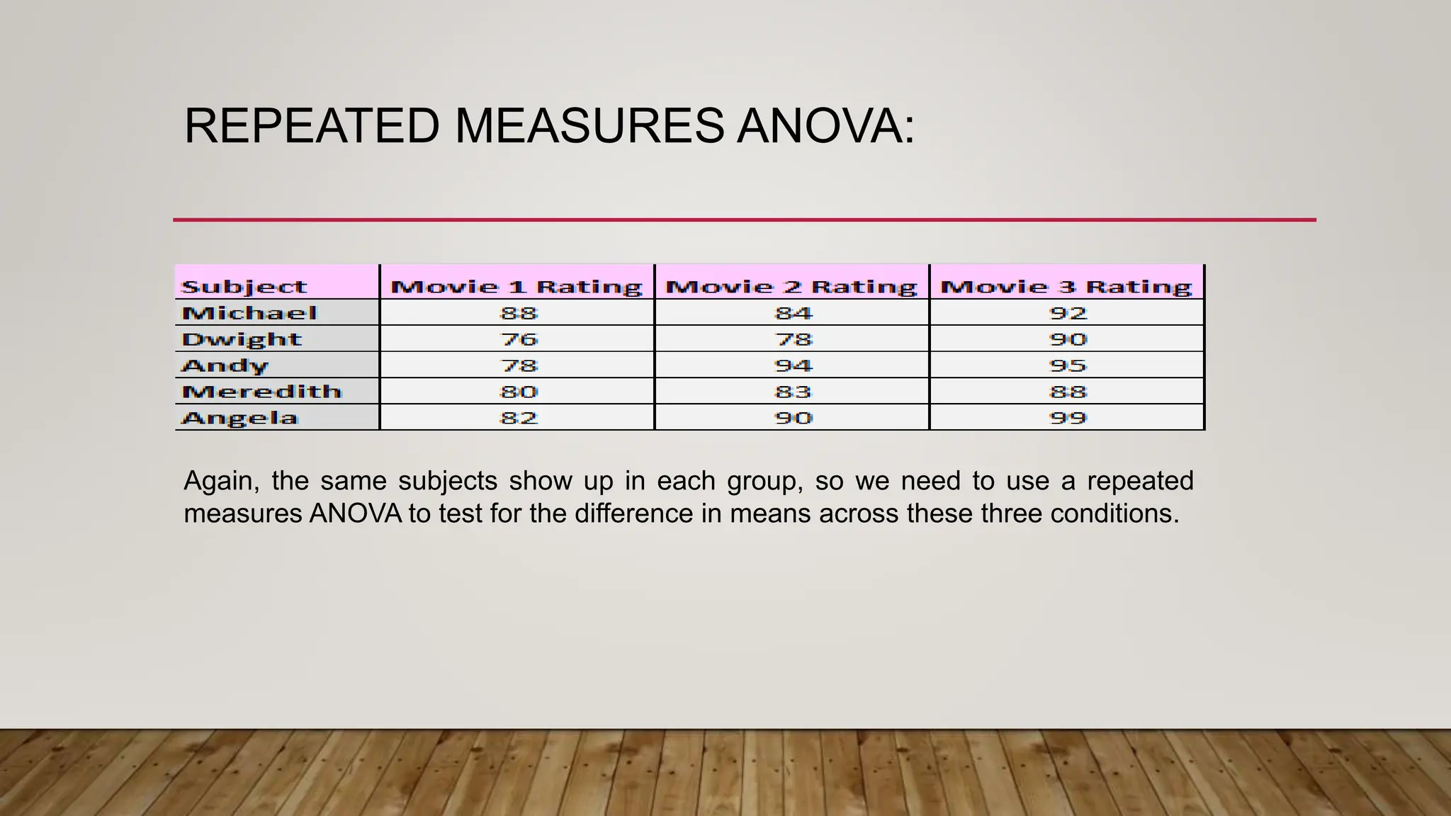
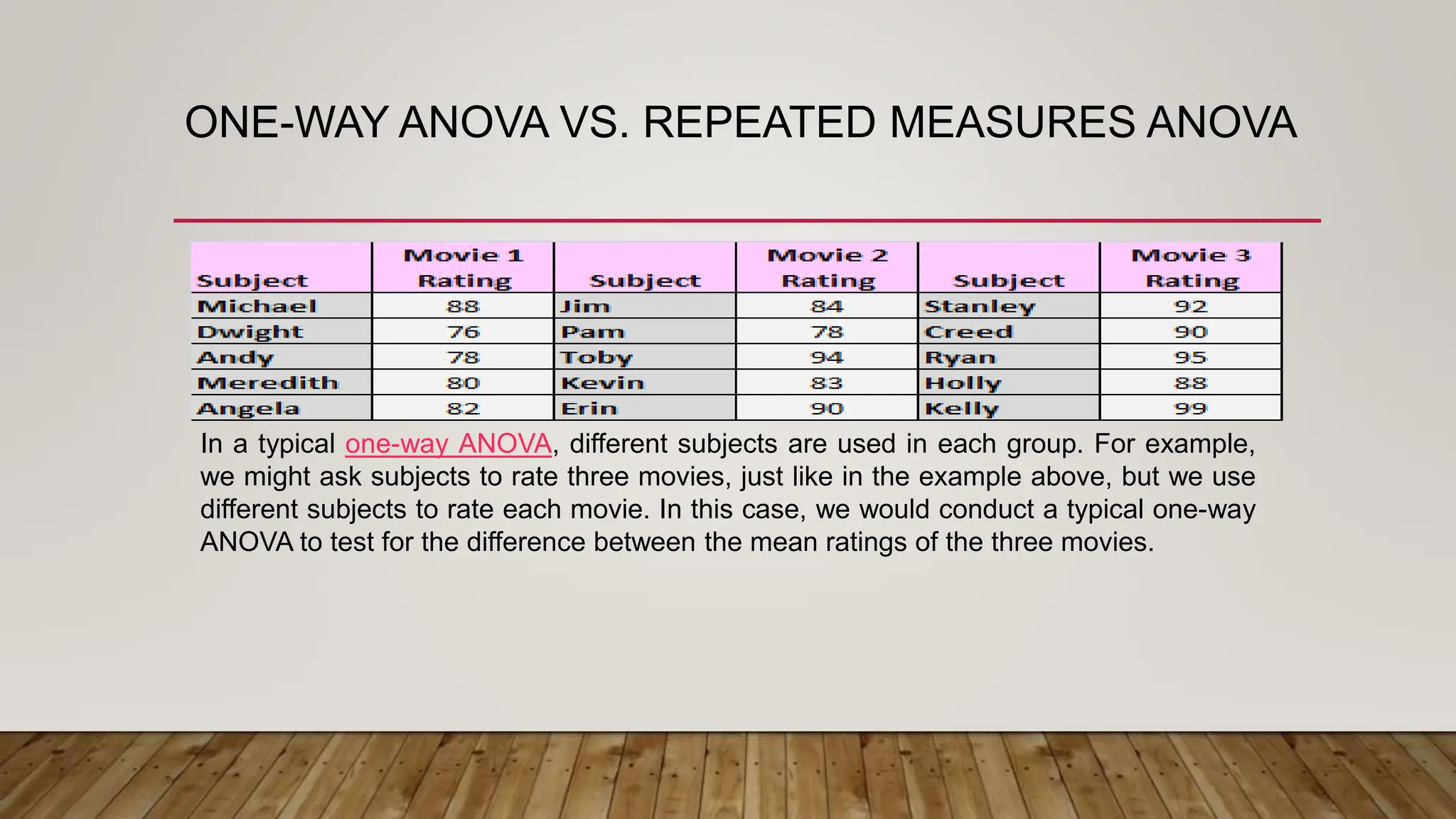
ONLINE WORKSHOP ON ADVANCE
STATISTICAL DATA ANALYSIS USING SPSS
Topic: Parametric Tests
Presented by
Borsha Neog
Assistant Professor
Assam Agricultural University, Jorhat-13
STATISTICAL INFERENCE:
• The main objective of sampling is to draw conclusions about the unknown population
from the information provided by a sample. This is called statistical inference.
• Statistical inference can be divided into two kinds: parameter estimation and
hypothesis testing.
• Parameter estimation is concerned with obtaining numerical values of the parameter
from a sample.
• Hypothesis testing is concerned with passing a judgement on some assumption
which we make (on the basis of some theory or information) about a true value of a
population parameter.
TESTS OF SIGNIFICANCE
A very important aspect of the sampling theory is the study of the tests of
significance, which enable us to decide on the basis of the sample results, if
(i) The deviation between the observed sample statistic and the hypothetical
parameter value, or
(ii) The deviation between two independent sample statistics; is significant or
might be attributed to chance or the fluctuations of sampling
NULL AND ALTERNATIVE HYPOTHESES
A definite statement about the population parameter. Such a hypothesis, which is
usually a hypothesis of no difference, is called null hypothesis and is usually
denoted by H0 .
According to Prof. R. A. Fisher, null hypothesis is the hypothesis which is tested for
possible rejection under the assumption that it is true.
• Any hypothesis which is complementary to the null hypothesis is called an
alternative hypothesis, usually denoted by H1.
NULL AND ALTERNATIVE HYPOTHESES
For example, if we want to test the null hypothesis that the population has a specified mean µ0
(say), i.e., H0:µ= µ0
Then the alternative hypothesis could be:
(i) H1: µ≠ µ0(i.e., µ> µ0 Or µ <µ0)
(ii) H1: µ> µ0
(iii) H1: µ <µ0
The alternative hypothesis in (i) is known as a two tailed alternative and the alternatives in (ii) and
(iii) are known as right tailed and left tailed alternatives repectively. The setting of alternative
hypothesis is very important since it enables us to decide whether we have to use a single
tailed (right or left) or two tailed test
ERRORS IN SAMPLING
The main objective in sampling theory is to draw valid inferences about the population
parameters on the basis of the sample results. As such we are liable to commit the
following two types of errors:
Type I error: reject H0 When it is true
Type II error: accept H0 When it is wrong, i.e., accept H0 When H1 is true.
In practice, type I error amounts to rejecting a lot when it is good and type II error may
be regarded as accepting the lot when it is bad.
Thus P( Reject a lot when it is good)= α
P( Accept a lot when it is bad)=β
CRITICAL REGION AND LEVEL OF
SIGNIFICANCE
A region which amounts to rejection of H0 is termed as critical region of rejection.
The probability α is known as the level of significance. In other words, level of
significance is the size of the type I error.
The level of significance usually employed in testing of hypothesis are 5% and 1%.
The level of significance is always fixed in advance before collecting the sample
information.
A significance level .05 indicates a 5% risk of concluding that a difference exists
when there is no actual difference.
CRITICAL VALUES OR SIGNIFICANT VALUES
The value of test statistic which separates the critical(or rejection) region and the
acceptance region is called the critical value or significant value. It depends on
(i) The level of significance used and
(ii) The alternative hypothesis, whether it is a two tailed or single tailed.
PROCEDURE FOR TESTING OF HYPOTHESIS
The various steps in testing of a statistical hypothesis are given below
1. Null hypothesis: set up the Null Hypothesis H0
2. Alternative hypothesis: set up the Alternative Hypothesis H1
This will enable us to decide whether we have to use a single tailed test or two tailed test.
3. Level of Significance: Choose the appropriate level of significance (α) depending on the
reliability of the estimates and permissible risk. This is to be decided before sample is drawn,
i.e., α is fixed in advance.
4. Test statistic: compute the test statistic
5. conclusion: compare the computed value of the test statistic with the statistical table value. If
the calculated value is less than the table value then null hypothesis become not significant.
Otherwise hypothesis is significant.
P VALUE IN STATISTICS:
• The p value, or probability value, tells you how likely it is that your data could
have occurred under the null hypothesis or describes how likely you are to have
found a particular set of observations if the null hypothesis were true.
• P values are used in hypothesis testing to help decide whether to reject the null
hypothesis. The smaller the p value, the more likely you are to reject the null
hypothesis.
T TEST:
• Student's t-test is a method of testing hypotheses about the mean of a small
sample drawn from a normally distributed population when the population
standard deviation is unknown.
• The family of t-tests falls in the category of parametric statistical tests where the
mean value(s) is (are) compared against a hypothesized value.
• Most frequently used t-tests are: For comparison of mean in single sample; two
samples related; two samples unrelated tests; more than two samples and testing
of correlation coefficient and regression coefficient against a hypothesized value
which is usually zero.
• In one-sample location test, it is tested whether or not the mean of the population has a
value as specified in a null hypothesis.
• In two independent sample location test, equality of means of two populations is tested.
• To compare the mean (difference between two related samples) against hypothesized
value of zero in a null hypothesis, also known as paired t-test or repeated-measures t-
test;
• To test whether or not correlation coefficient, the slope of a regression line differs
significantly from zero.
T-TEST FOR ONE SAMPLE
Suppose we want to test:
If a random sample xi(i =1,2,…,n) of size n has been drawn from a normal
population with a specified mean µ0
Or if the sample mean differs significantly from the hypothetical value µ0 of the
population mean.
Under the null hypothesis, H0
The sample has been drawn from the population with mean µ0
Or there is no significant difference between the sample mean and the population
mean.
T-TEST FOR ONE SAMPLE
• For example, in a random sample of 30 hypertensive males, the observed mean
body mass index (BMI) is 27.0 kg/m 2 and the standard deviation is 4.0. Also,
suppose it is known that the mean BMI in no hypertensive males is 25 kg/m 2. If
the question is to know whether or not these 30 observations could have come
from a population with a mean of 25 kg/m 2. To determine this, one sample t-test
is used with the null hypothesis H0: Mean = 25, against alternate hypothesis of
H1: Mean ≠ 25. Since the standard deviation of the hypothesized population is
not known, therefore, t-test would be appropriate; otherwise, Z-test would have
been used
ASSUMPTIONS FOR STUDENT’S T TEST
• The parent population from which the sample is drawn is normal.
• The sample observations are independent, i.e., the sample is random.
• The population standard deviation σ is unknown.
T TEST FOR DIFFERENCE OF MEANS
• Suppose we want to test if two independent samples xi (i=1,2,…,n1) and
yj(j=1,2,…,n2) of sizes n1 and n2 have been drawn from two normal
populations with means µx and µy respectively.
• Under the null hypothesis that the samples have been drawn from the
normal populations with means µx and µy and under the assumption that
the population variance are equal, i.e., σx
2= σy
2
T-TEST FOR TWO INDEPENDENT SAMPLES:
• To test the null hypothesis that the means of two populations are equal;
Student's t-test is used provided the variances of the two populations are equal
and the two samples are assumed to be random sample. When this assumption
of equality of variance is not fulfilled, the form of the test used is a modified t-test.
These tests are also known as two-sample independent t-tests with equal
variance or unequal variance, respectively.
PAIRED T TEST FOR DIFFERENCE OF MEANS
• Let us now consider the case when the sample sizes are equal, i.e., n1 = n2 = n(say) and
the two samples are not independent but the sample observations are paired
together. The problem is to test if the sample means differ significant or not.
• For example, suppose we want to test the efficacy of a particular drug, say, for inducing
sleep. Let xi and yi(i=1,2,…,n) be the readings, in hours of sleep, on the ith individual,
before and after the drug is given respectively.
• Here we consider the increments,
di= xi- yi
Under the null hypothesis, increments are due to fluctuations of sampling, i.e., the drug
is not responsible for these increments.
•
PAIRED T TEST :
• Two samples can be regarded as related in a pre- and post-design (self-pairing).
In a pre- and post–design, each subject is used as his or her own control. For
example, an investigator wants to assess effect of an intervention in reducing
systolic blood pressure (SBP) in a pre- and post-design. Here, for each patient,
there would be two observations of SBP, that is, before and after. where the null
hypothesis would be to test the mean difference in SBP equal to zero against the
alternate hypothesis of mean SBP being not equal to zero. The underlying
assumption for using paired t-test is that under the null hypothesis the population
of difference in normally distributed and this can be judged using the sample
values.
T-TEST FOR SEVERAL MEANS ( ONE WAY
ANOVA):
• When there are more than two groups, use of multiple t-test (for each pair of
groups) is incorrect because it may give false-positive result, hence, in such
situations, one-way analysis of variance (ANOVA), followed by multiple
comparisons (post-hoc ANOVA), if required, is used to test the equality of more
than two means as the null hypothesis.
REPEATED MEASURES ANOVA:
• A repeated measures ANOVA is used to determine whether or not there is a
statistically significant difference between the means of three or more groups in
which the same subjects show up in each group.
• A repeated measures ANOVA is typically used in two specific situations:
• 1. Measuring the mean scores of subjects during three or more time
points. For example, you might want to measure the resting heart rate of subjects
one month before they start a training program, during the middle of the training
program, and one month after the training program to see if there is a significant
difference in mean resting heart rate across these three time points.
REPEATED MEASURES ANOVA:
Notice how the same subjects show up at each time point.
We repeatedly measured the same subjects, hence the reason why we used a
repeated measures ANOVA.
2. Measuring the mean scores of subjects under three different conditions.
For example, you might have subjects watch three different movies and rate each
one based on how much they enjoyed it.
REPEATED MEASURES ANOVA:
Again, the same subjects show up in each group, so we need to use a repeated
measures ANOVA to test for the difference in means across these three conditions.
ONE-WAY ANOVA VS. REPEATED MEASURES ANOVA
In a typical one-way ANOVA, different subjects are used in each group. For example,
we might ask subjects to rate three movies, just like in the example above, but we use
different subjects to rate each movie. In this case, we would conduct a typical one-way
ANOVA to test for the difference between the mean ratings of the three movies.
THANK YOU

Day-2_Presentation for SPSS parametric workshop.pptx

  • 1.
    ONLINE WORKSHOP ONADVANCE STATISTICAL DATA ANALYSIS USING SPSS Topic: Parametric Tests Presented by Borsha Neog Assistant Professor Assam Agricultural University, Jorhat-13
  • 2.
    STATISTICAL INFERENCE: • Themain objective of sampling is to draw conclusions about the unknown population from the information provided by a sample. This is called statistical inference. • Statistical inference can be divided into two kinds: parameter estimation and hypothesis testing. • Parameter estimation is concerned with obtaining numerical values of the parameter from a sample. • Hypothesis testing is concerned with passing a judgement on some assumption which we make (on the basis of some theory or information) about a true value of a population parameter.
  • 3.
    TESTS OF SIGNIFICANCE Avery important aspect of the sampling theory is the study of the tests of significance, which enable us to decide on the basis of the sample results, if (i) The deviation between the observed sample statistic and the hypothetical parameter value, or (ii) The deviation between two independent sample statistics; is significant or might be attributed to chance or the fluctuations of sampling
  • 4.
    NULL AND ALTERNATIVEHYPOTHESES A definite statement about the population parameter. Such a hypothesis, which is usually a hypothesis of no difference, is called null hypothesis and is usually denoted by H0 . According to Prof. R. A. Fisher, null hypothesis is the hypothesis which is tested for possible rejection under the assumption that it is true. • Any hypothesis which is complementary to the null hypothesis is called an alternative hypothesis, usually denoted by H1.
  • 5.
    NULL AND ALTERNATIVEHYPOTHESES For example, if we want to test the null hypothesis that the population has a specified mean µ0 (say), i.e., H0:µ= µ0 Then the alternative hypothesis could be: (i) H1: µ≠ µ0(i.e., µ> µ0 Or µ <µ0) (ii) H1: µ> µ0 (iii) H1: µ <µ0 The alternative hypothesis in (i) is known as a two tailed alternative and the alternatives in (ii) and (iii) are known as right tailed and left tailed alternatives repectively. The setting of alternative hypothesis is very important since it enables us to decide whether we have to use a single tailed (right or left) or two tailed test
  • 6.
    ERRORS IN SAMPLING Themain objective in sampling theory is to draw valid inferences about the population parameters on the basis of the sample results. As such we are liable to commit the following two types of errors: Type I error: reject H0 When it is true Type II error: accept H0 When it is wrong, i.e., accept H0 When H1 is true. In practice, type I error amounts to rejecting a lot when it is good and type II error may be regarded as accepting the lot when it is bad. Thus P( Reject a lot when it is good)= α P( Accept a lot when it is bad)=β
  • 7.
    CRITICAL REGION ANDLEVEL OF SIGNIFICANCE A region which amounts to rejection of H0 is termed as critical region of rejection. The probability α is known as the level of significance. In other words, level of significance is the size of the type I error. The level of significance usually employed in testing of hypothesis are 5% and 1%. The level of significance is always fixed in advance before collecting the sample information. A significance level .05 indicates a 5% risk of concluding that a difference exists when there is no actual difference.
  • 8.
    CRITICAL VALUES ORSIGNIFICANT VALUES The value of test statistic which separates the critical(or rejection) region and the acceptance region is called the critical value or significant value. It depends on (i) The level of significance used and (ii) The alternative hypothesis, whether it is a two tailed or single tailed.
  • 9.
    PROCEDURE FOR TESTINGOF HYPOTHESIS The various steps in testing of a statistical hypothesis are given below 1. Null hypothesis: set up the Null Hypothesis H0 2. Alternative hypothesis: set up the Alternative Hypothesis H1 This will enable us to decide whether we have to use a single tailed test or two tailed test. 3. Level of Significance: Choose the appropriate level of significance (α) depending on the reliability of the estimates and permissible risk. This is to be decided before sample is drawn, i.e., α is fixed in advance. 4. Test statistic: compute the test statistic 5. conclusion: compare the computed value of the test statistic with the statistical table value. If the calculated value is less than the table value then null hypothesis become not significant. Otherwise hypothesis is significant.
  • 10.
    P VALUE INSTATISTICS: • The p value, or probability value, tells you how likely it is that your data could have occurred under the null hypothesis or describes how likely you are to have found a particular set of observations if the null hypothesis were true. • P values are used in hypothesis testing to help decide whether to reject the null hypothesis. The smaller the p value, the more likely you are to reject the null hypothesis.
  • 12.
    T TEST: • Student'st-test is a method of testing hypotheses about the mean of a small sample drawn from a normally distributed population when the population standard deviation is unknown. • The family of t-tests falls in the category of parametric statistical tests where the mean value(s) is (are) compared against a hypothesized value. • Most frequently used t-tests are: For comparison of mean in single sample; two samples related; two samples unrelated tests; more than two samples and testing of correlation coefficient and regression coefficient against a hypothesized value which is usually zero.
  • 13.
    • In one-samplelocation test, it is tested whether or not the mean of the population has a value as specified in a null hypothesis. • In two independent sample location test, equality of means of two populations is tested. • To compare the mean (difference between two related samples) against hypothesized value of zero in a null hypothesis, also known as paired t-test or repeated-measures t- test; • To test whether or not correlation coefficient, the slope of a regression line differs significantly from zero.
  • 14.
    T-TEST FOR ONESAMPLE Suppose we want to test: If a random sample xi(i =1,2,…,n) of size n has been drawn from a normal population with a specified mean µ0 Or if the sample mean differs significantly from the hypothetical value µ0 of the population mean. Under the null hypothesis, H0 The sample has been drawn from the population with mean µ0 Or there is no significant difference between the sample mean and the population mean.
  • 15.
    T-TEST FOR ONESAMPLE • For example, in a random sample of 30 hypertensive males, the observed mean body mass index (BMI) is 27.0 kg/m 2 and the standard deviation is 4.0. Also, suppose it is known that the mean BMI in no hypertensive males is 25 kg/m 2. If the question is to know whether or not these 30 observations could have come from a population with a mean of 25 kg/m 2. To determine this, one sample t-test is used with the null hypothesis H0: Mean = 25, against alternate hypothesis of H1: Mean ≠ 25. Since the standard deviation of the hypothesized population is not known, therefore, t-test would be appropriate; otherwise, Z-test would have been used
  • 16.
    ASSUMPTIONS FOR STUDENT’ST TEST • The parent population from which the sample is drawn is normal. • The sample observations are independent, i.e., the sample is random. • The population standard deviation σ is unknown.
  • 17.
    T TEST FORDIFFERENCE OF MEANS • Suppose we want to test if two independent samples xi (i=1,2,…,n1) and yj(j=1,2,…,n2) of sizes n1 and n2 have been drawn from two normal populations with means µx and µy respectively. • Under the null hypothesis that the samples have been drawn from the normal populations with means µx and µy and under the assumption that the population variance are equal, i.e., σx 2= σy 2
  • 18.
    T-TEST FOR TWOINDEPENDENT SAMPLES: • To test the null hypothesis that the means of two populations are equal; Student's t-test is used provided the variances of the two populations are equal and the two samples are assumed to be random sample. When this assumption of equality of variance is not fulfilled, the form of the test used is a modified t-test. These tests are also known as two-sample independent t-tests with equal variance or unequal variance, respectively.
  • 19.
    PAIRED T TESTFOR DIFFERENCE OF MEANS • Let us now consider the case when the sample sizes are equal, i.e., n1 = n2 = n(say) and the two samples are not independent but the sample observations are paired together. The problem is to test if the sample means differ significant or not. • For example, suppose we want to test the efficacy of a particular drug, say, for inducing sleep. Let xi and yi(i=1,2,…,n) be the readings, in hours of sleep, on the ith individual, before and after the drug is given respectively. • Here we consider the increments, di= xi- yi Under the null hypothesis, increments are due to fluctuations of sampling, i.e., the drug is not responsible for these increments. •
  • 20.
    PAIRED T TEST: • Two samples can be regarded as related in a pre- and post-design (self-pairing). In a pre- and post–design, each subject is used as his or her own control. For example, an investigator wants to assess effect of an intervention in reducing systolic blood pressure (SBP) in a pre- and post-design. Here, for each patient, there would be two observations of SBP, that is, before and after. where the null hypothesis would be to test the mean difference in SBP equal to zero against the alternate hypothesis of mean SBP being not equal to zero. The underlying assumption for using paired t-test is that under the null hypothesis the population of difference in normally distributed and this can be judged using the sample values.
  • 21.
    T-TEST FOR SEVERALMEANS ( ONE WAY ANOVA): • When there are more than two groups, use of multiple t-test (for each pair of groups) is incorrect because it may give false-positive result, hence, in such situations, one-way analysis of variance (ANOVA), followed by multiple comparisons (post-hoc ANOVA), if required, is used to test the equality of more than two means as the null hypothesis.
  • 22.
    REPEATED MEASURES ANOVA: •A repeated measures ANOVA is used to determine whether or not there is a statistically significant difference between the means of three or more groups in which the same subjects show up in each group. • A repeated measures ANOVA is typically used in two specific situations: • 1. Measuring the mean scores of subjects during three or more time points. For example, you might want to measure the resting heart rate of subjects one month before they start a training program, during the middle of the training program, and one month after the training program to see if there is a significant difference in mean resting heart rate across these three time points.
  • 23.
  • 24.
    REPEATED MEASURES ANOVA: Noticehow the same subjects show up at each time point. We repeatedly measured the same subjects, hence the reason why we used a repeated measures ANOVA. 2. Measuring the mean scores of subjects under three different conditions. For example, you might have subjects watch three different movies and rate each one based on how much they enjoyed it.
  • 25.
    REPEATED MEASURES ANOVA: Again,the same subjects show up in each group, so we need to use a repeated measures ANOVA to test for the difference in means across these three conditions.
  • 26.
    ONE-WAY ANOVA VS.REPEATED MEASURES ANOVA In a typical one-way ANOVA, different subjects are used in each group. For example, we might ask subjects to rate three movies, just like in the example above, but we use different subjects to rate each movie. In this case, we would conduct a typical one-way ANOVA to test for the difference between the mean ratings of the three movies.
  • 27.