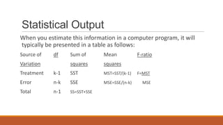
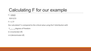
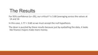
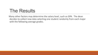
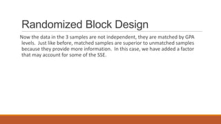
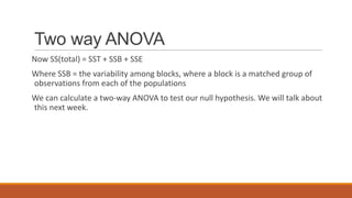
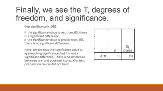
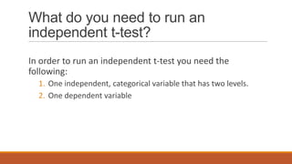
The document describes experimental designs and statistical tests used to analyze data from experiments with multiple groups. It discusses paired t-tests, independent t-tests, and analysis of variance (ANOVA). For ANOVA, it provides an example to calculate sum of squares for treatment (SST), sum of squares for error (SSE), and the F-statistic. The example shows applying a one-way ANOVA to compare average incomes of accounting, marketing and finance majors. It finds no significant difference between the groups. A randomized block design is then proposed to account for variability from GPA levels.

1. Experimental Design
Data analysis
GROUP 5

2. PAIRED T-TEST
PRESENTER: TRAN THI NGAN GIANG

3. Introduction
A paired t-test is used to compare two population means where you have two samples in which
observations in one sample can be paired with observations in the other sample.
For example:
A diagnostic test was made before studying a particular module and then again after completing
the module. We want to find out if, in general, our teaching leads to improvements in students’
knowledge/skills.

4. First, we see the descriptive statistics for
both variables.
The post-test mean scores are higher.

5. Next, we see the correlation between
the two variables.
There is a strong positive correlation. People who did well on the pre-test
also did well on the post-test.

6. Finally, we see the T, degrees of
freedom, and significance.
Our significance is .053
If the significance value is less than .05, there
is a significant difference.
If the significance value is greater than. 05,
there is no significant difference.
Here, we see that the significance value is
approaching significance, but it is not a
significant difference. There is no difference
between pre- and post-test scores. Our test
preparation course did not help!

7. INDEPENDENT SAMPLES
T-TESTS
PRESENTER: DINH QUOC MINH DANG

8. Outline
1. Introduction
2. Hypothesis for the independent t-test
3. What do you need to run an independent t-test?
4. Formula
5. Example (Calculating + Reporting)

9. Introduction
The independent t-test, also called the two sample t-test or
student's t-test is an inferential statistical test that determines
whether there is a statistically significant difference between the
means in two unrelated groups.

10. Hypothesis for the independent t-test
The null hypothesis for the independent t-test is that the population means from the
two unrelated groups are equal:
H0: u1 = u2
In most cases, we are looking to see if we can show that we can reject the null
hypothesis and accept the alternative hypothesis, which is that the population means
are not equal:
HA: u1 ≠ u2
To do this we need to set a significance level (alpha) that allows us to either reject or
accept the alternative hypothesis. Most commonly, this value is set at 0.05.

11. What do you need to run an
independent t-test?
In order to run an independent t-test you need the
following:
1. One independent, categorical variable that has two levels.
2. One dependent variable

12. Formula
M: mean (the average score of the group)
SD: Standard Deviation
N: number of scores in each group
Exp: Experimental Group
Con: Control Group

13. Formula

14. Example

15. Example

16. Effect Size

17. Reporting the Result of an
Independent T-Test
When reporting the result of an independent t-test, you
need to include the t-statistic value, the degrees of freedom
(df) and the significance value of the test (P-value). The
format of the test result is: t(df) = t-statistic, P = significance
value.

18. Example result (APA Style)
An independent samples T-test is presented the same as the one-sample t-test:
t(75) = 2.11, p = .02 (one –tailed), d = .48
Degrees of
freedom Value of
statistic Include if test is Effect size if
Significance of one-tailed available
statistic
Example: Survey respondents who were employed by the federal, state, or local government
had significantly higher socioeconomic indices (M = 55.42, SD = 19.25) than survey
respondents who were employed by a private employer (M = 47.54, SD = 18.94) , t(255) =
2.363, p = .01 (one-tailed).

19. Analysis of Variance
(ANOVA)
PRESENTER : MINH SANG

20. Introduction
We already learned about the chi square test for independence, which is useful for data that is
measured at the nominal or ordinal level of analysis.
If we have data measured at the interval level, we can compare two or more population groups
in terms of their population means using a technique called analysis of variance, or ANOVA.

21. Completely randomized design
Population 1 Population 2….. Population k
Mean = 1 Mean = 2 …. Mean = k
Variance= 2 Variance= 2 … Variance = 2
1 2 k
We want to know something about how the populations compare.
Do they have the same mean? We can collect random samples from
each population, which gives us the following data.

22. Completely randomized design
Mean = M1 Mean = M2 ..… Mean = Mk
Variance=s12 Variance=s22 …. Variance = sk2
N1 cases N2 cases …. Nk cases
Suppose we want to compare 3 college majors in a business school
by the average annual income people make 2 years after graduation.
We collect the following data (in $1000s) based on random surveys.

23. Completely randomized design
Accounting Marketing Finance
27 23 48
22 36 35
33 27 46
25 44 36
38 39 28
29 32 29

24. Completely randomized design
Can the dean conclude that there are differences among the major’s incomes?
Ho : 1= 2= 3
HA: 1 2 3
In this problem we must take into account:
1) The variance between samples, or the actual differences by major.
This is called the sum of squares for treatment (SST).

25. Completely randomized design
2) The variance within samples, or the variance of incomes within a single major.
This is called the sum of squares for error (SSE).
Recall that when we sample, there will always be a chance of getting something
different than the population. We account for this through #2, or the SSE.

26. F-Statistic
For this test, we will calculate a F statistic, which is used to compare variances.
F = SST/(k-1)
SSE/(n-k)
SST=sum of squares for treatment
SSE=sum of squares for error
k = the number of populations
N = total sample size

27. F-statistic
Intuitively, the F statistic is:
F = explained variance
unexplained variance
Explained variance is the difference between majors
Unexplained variance is the difference based on random sampling for each group
(see Figure 10-1, page 327)

28. Calculating SST
SST = ni(Mi - )2
= grand mean or = Mi/k or the sum of all values for all groups divided by
total sample size
Mi = mean for each sample
k= the number of populations

29. Calculating SST
By major
Accounting M1=29, n1=6
Marketing M2=33.5, n2=6
Finance M3=37, n3=6
= (29+33.5+37)/3 = 33.17
SST = (6)(29-33.17)2 + (6)(33.5-33.17)2 + (6)(37-33.17)2 = 193

30. Calculating SST
Note that when M1 = M2 = M3, then SST=0 which would support the null
hypothesis.
In this example, the samples are of equal size, but we can also run this analysis
with samples of varying size also.

31. Calculating SSE
SSE = (Xit – Mi)2
In other words, it is just the variance for each sample added together.
SSE = (X1t – M1)2 + (X2t – M2)2 +
(X3t – M3)2
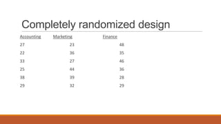
SSE = [(27-29)2 + (22-29)2 +…+ (29-29)2]
+ [(23-33.5)2 + (36-33.5)2 +…]
+ [(48-37)2 + (35-37)2 +…+ (29-37)2]
SSE = 819.5

32. Statistical Output
When you estimate this information in a computer program, it will
typically be presented in a table as follows:
Source of df Sum of Mean F-ratio
Variation squares squares
Treatment k-1 SST MST=SST/(k-1) F=MST
Error n-k SSE MSE=SSE/(n-k) MSE
Total n-1 SS=SST+SSE

33. Calculating F for our example
F = 193/2
819.5/15
F = 1.77
Our calculated F is compared to the critical value using the F-distribution with
F , k-1, n-k degrees of freedom
k-1 (numerator df)
n-k (denominator df)

34. The Results
For 95% confidence ( =.05), our critical F is 3.68 (averaging across the values at
14 and 16
In this case, 1.77 < 3.68 so we must accept the null hypothesis.
The dean is puzzled by these results because just by eyeballing the data, it looks
like finance majors make more money.

35. The Results
Many other factors may determine the salary level, such as GPA. The dean
decides to collect new data selecting one student randomly from each major
with the following average grades.

36. New data
Average Accounting Marketing Finance M(b)
A+ 41 45 51 M(b1)=45.67
A 36 38 45 M(b2)=39.67
B+ 27 33 31 M(b3)=30.83
B 32 29 35 M(b4)=32
C+ 26 31 32 M(b5)=29.67
C 23 25 27 M(b6)=25
M(t)1=30.83 M(t)2=33.5 M(t)3=36.83
= 33.72

37. Randomized Block Design
Now the data in the 3 samples are not independent, they are matched by GPA
levels. Just like before, matched samples are superior to unmatched samples
because they provide more information. In this case, we have added a factor
that may account for some of the SSE.

38. Two way ANOVA
Now SS(total) = SST + SSB + SSE
Where SSB = the variability among blocks, where a block is a matched group of
observations from each of the populations
We can calculate a two-way ANOVA to test our null hypothesis. We will talk about
this next week.