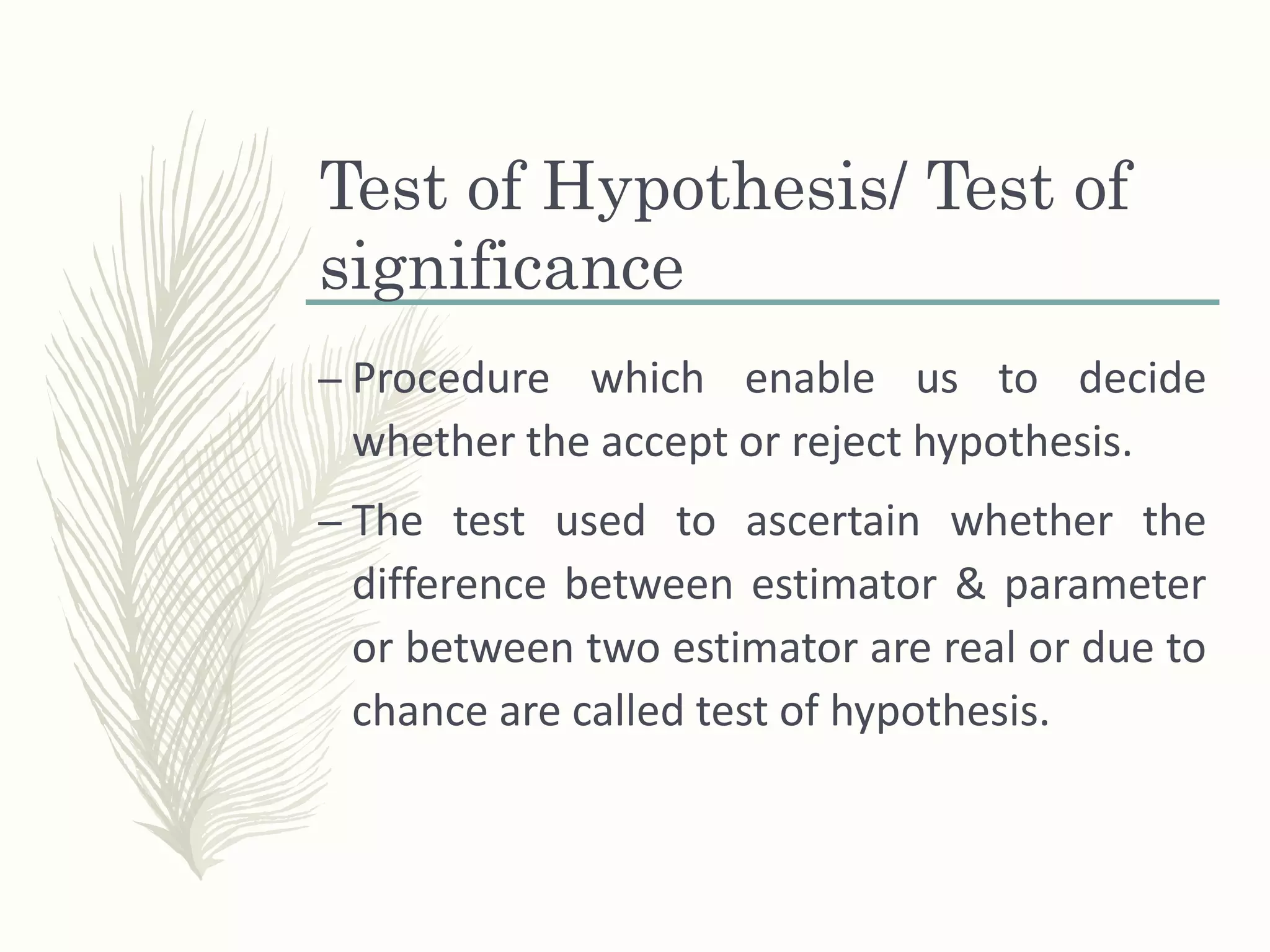
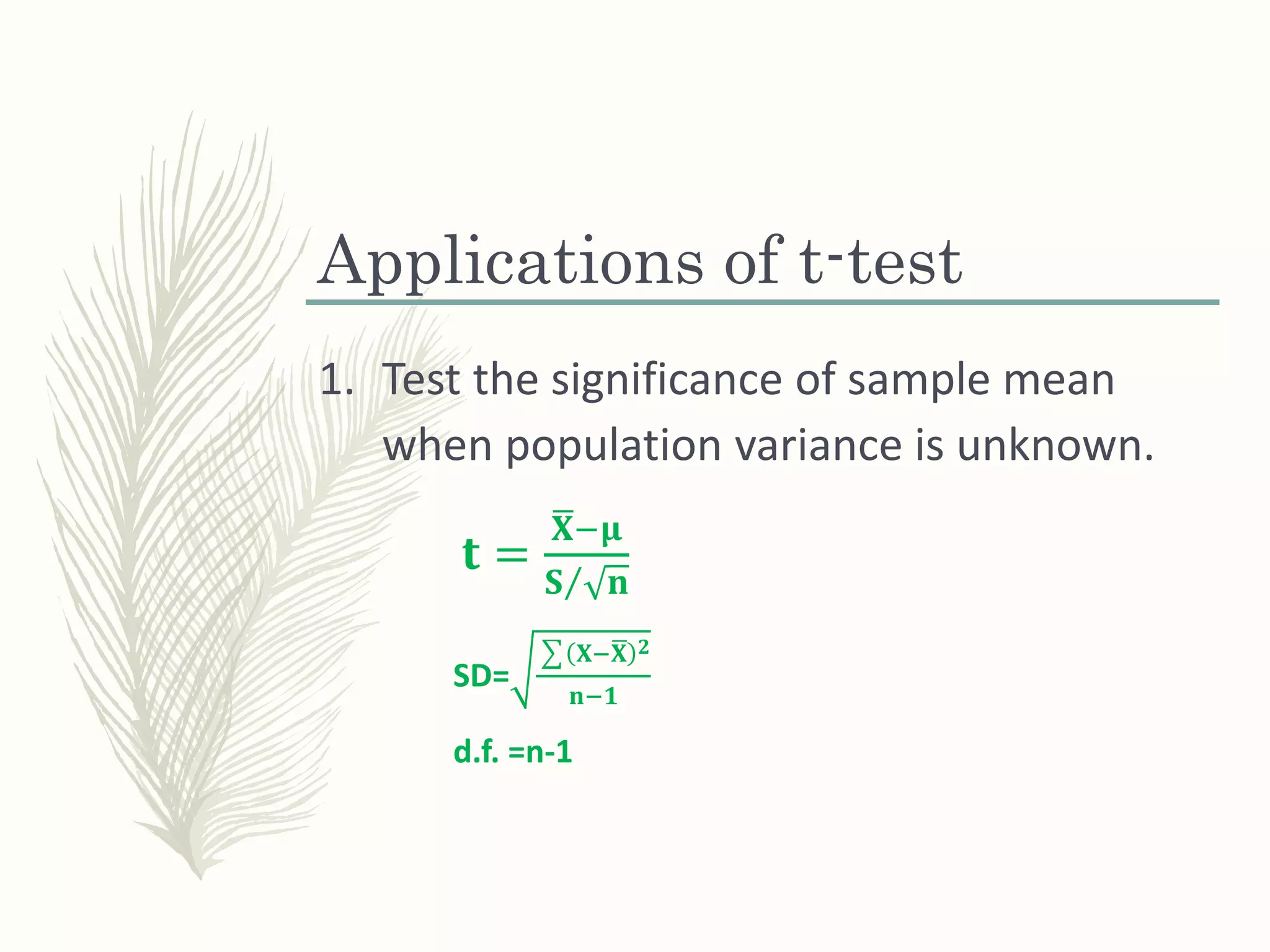
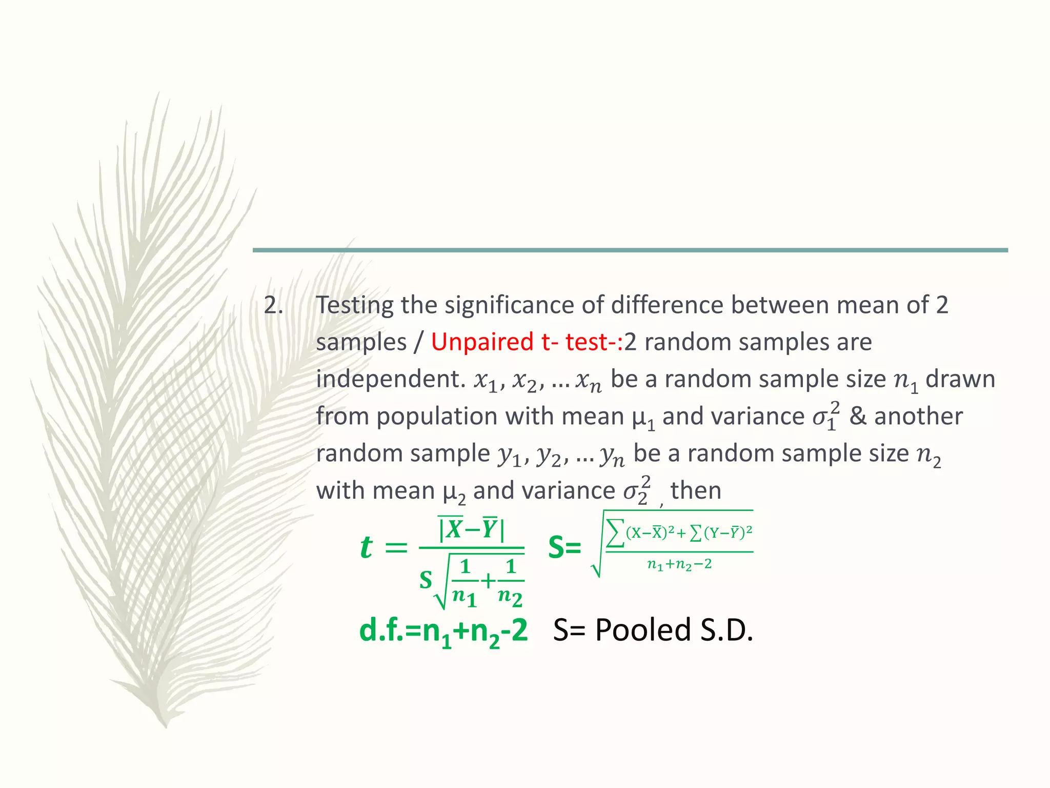
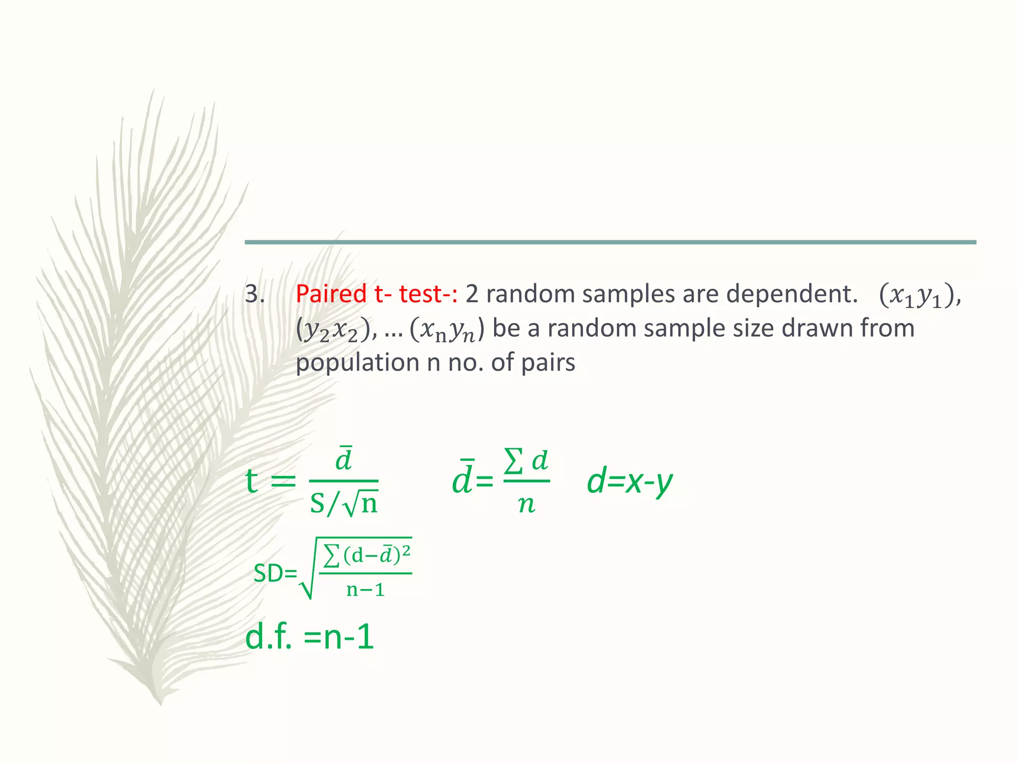
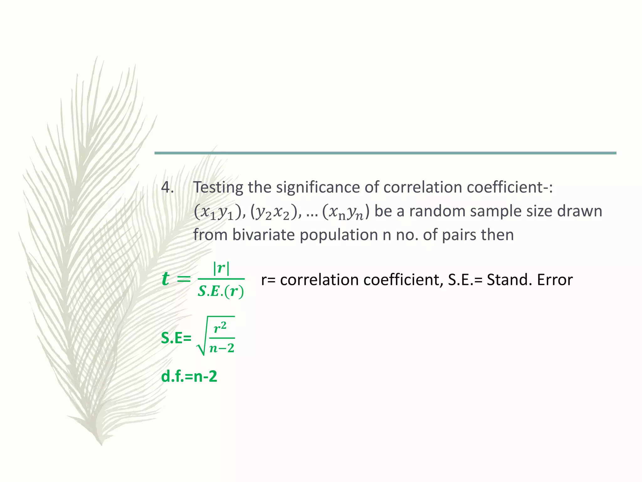
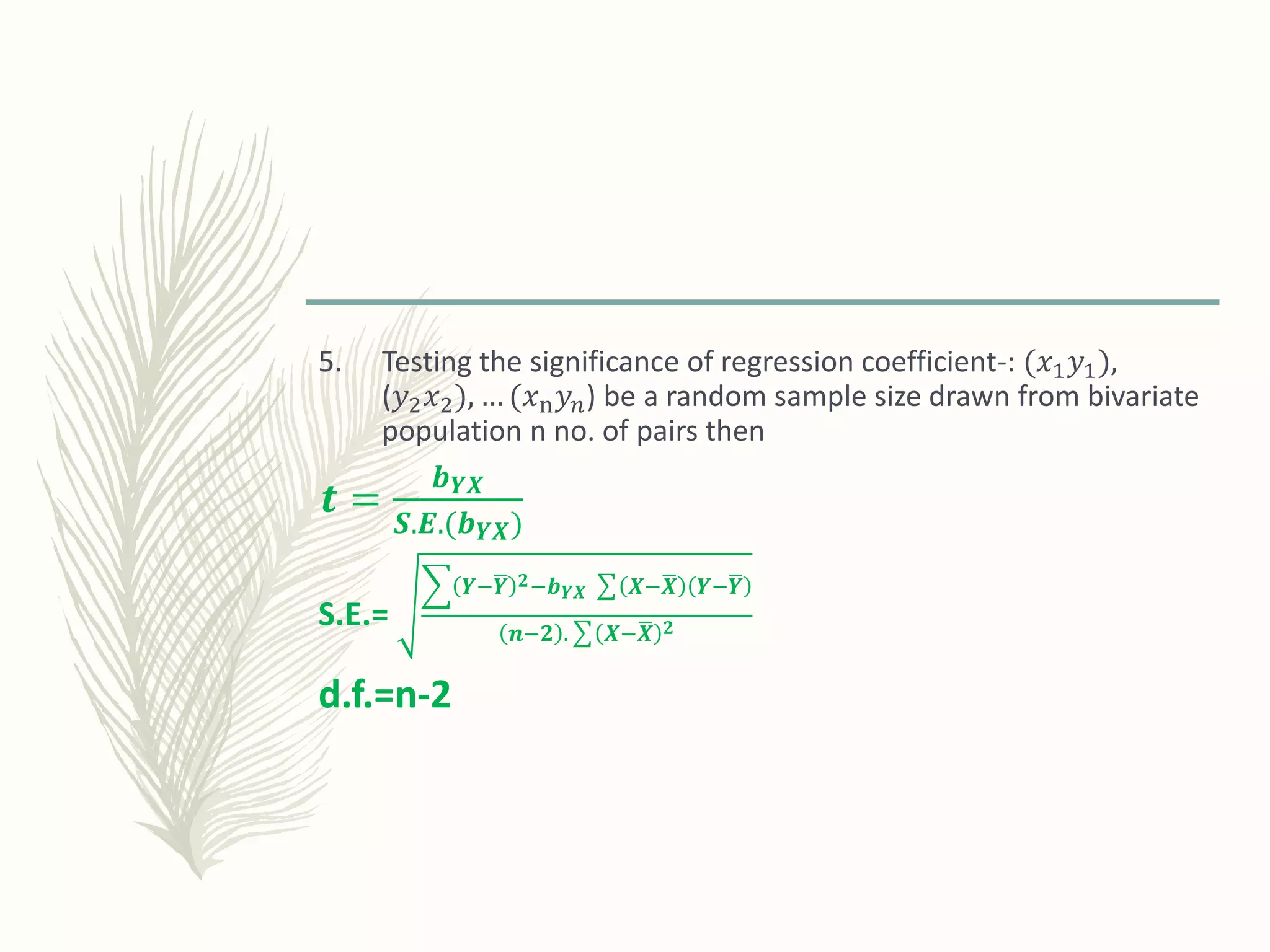
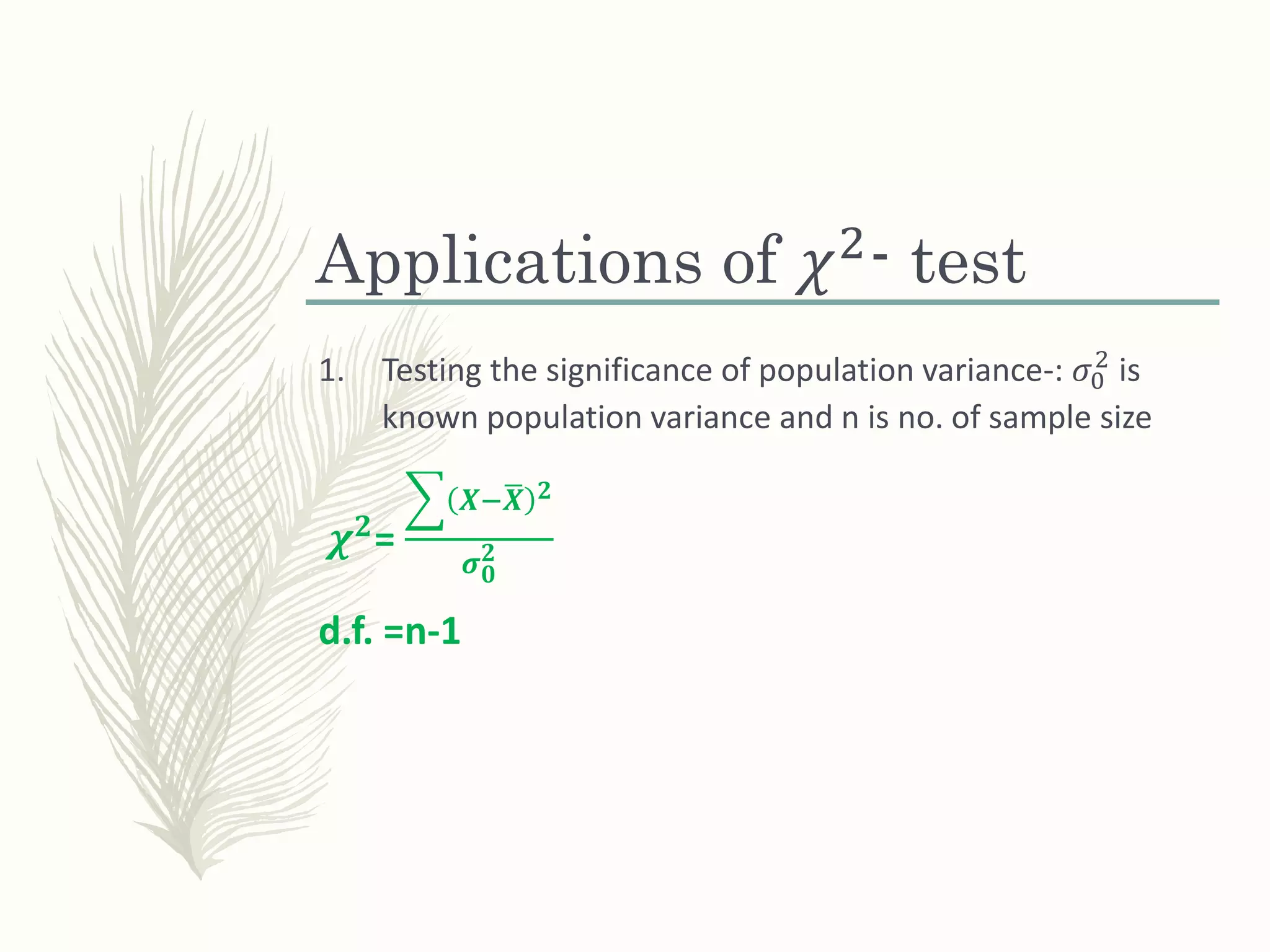
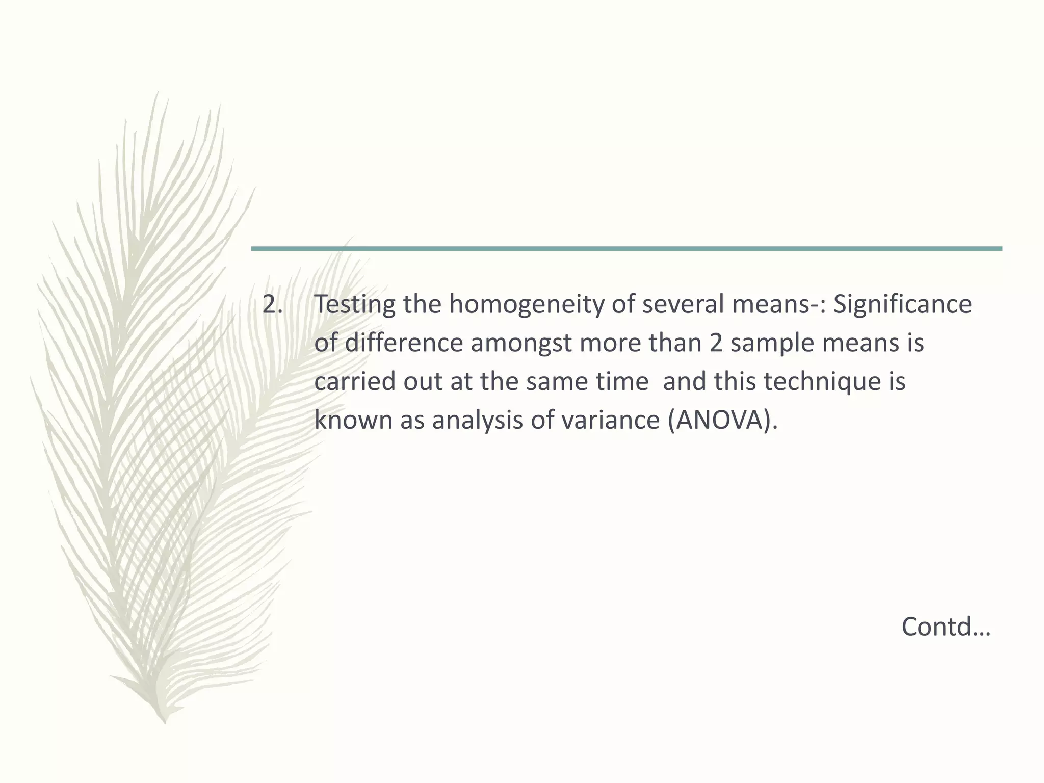
This document provides an overview of common statistical hypothesis tests including: 1) The t-test, which is used to test differences between sample means and the significance of sample means. 2) The chi-square test, which evaluates differences between observed and expected frequencies without distributional assumptions. It is used for goodness of fit tests and tests of independence. 3) Analysis of variance (ANOVA), which tests for differences among two or more means by analyzing variance estimates. It is used to evaluate whether experimental factors have significant effects on outcomes. 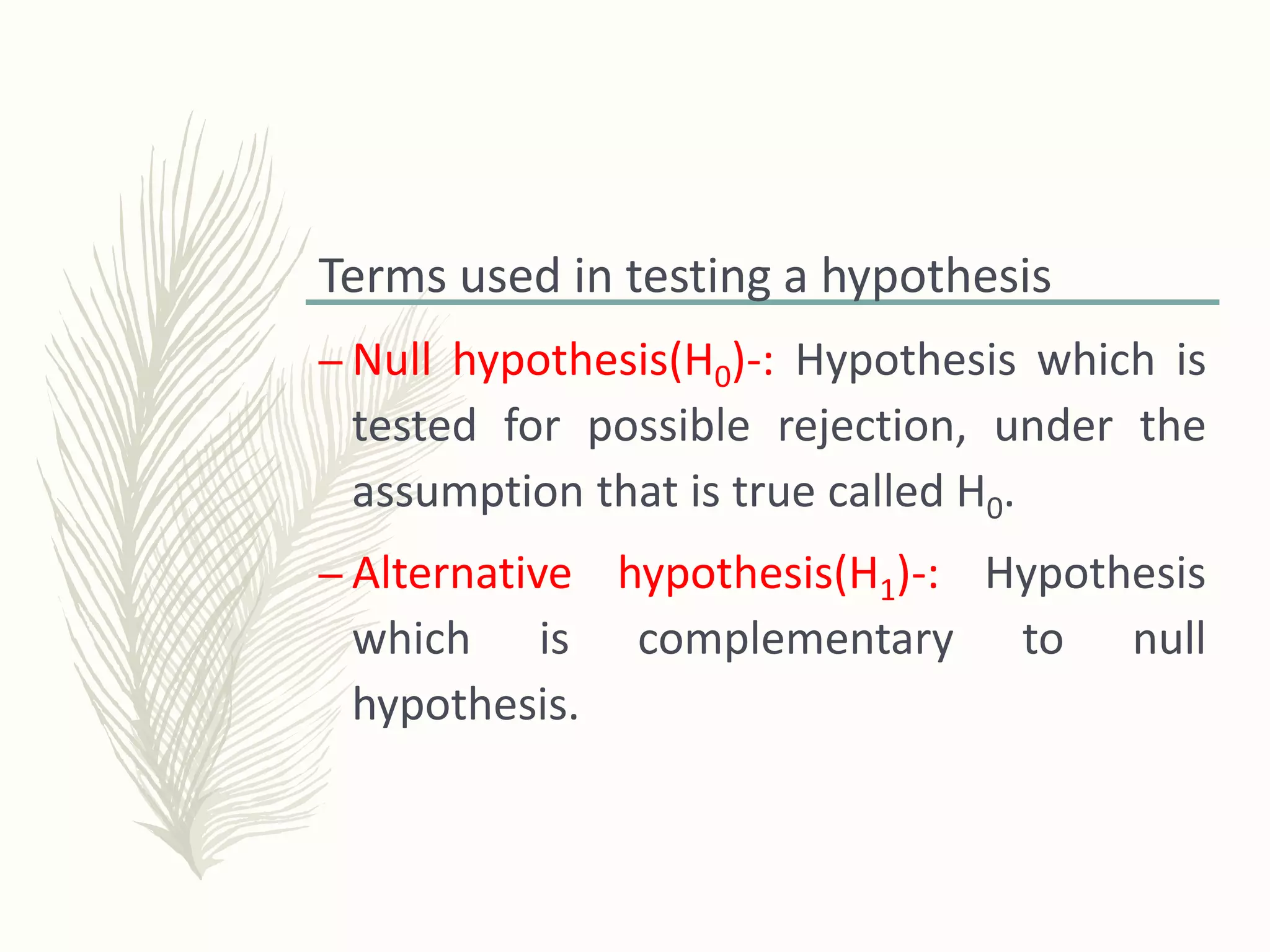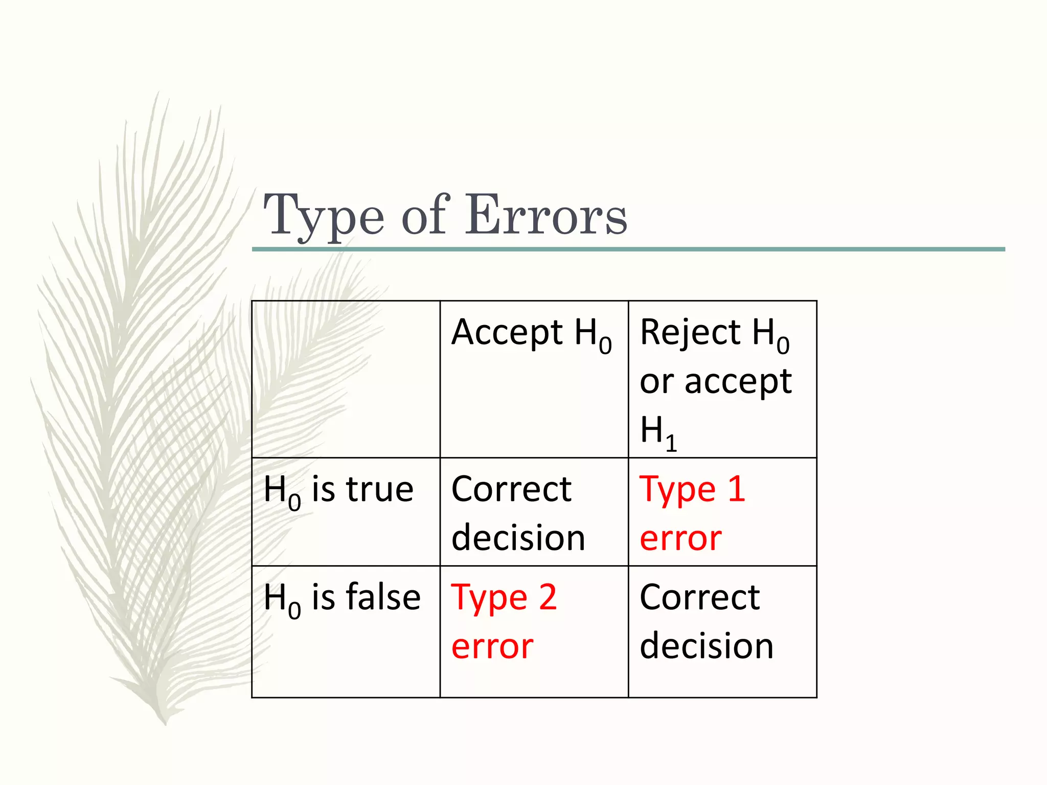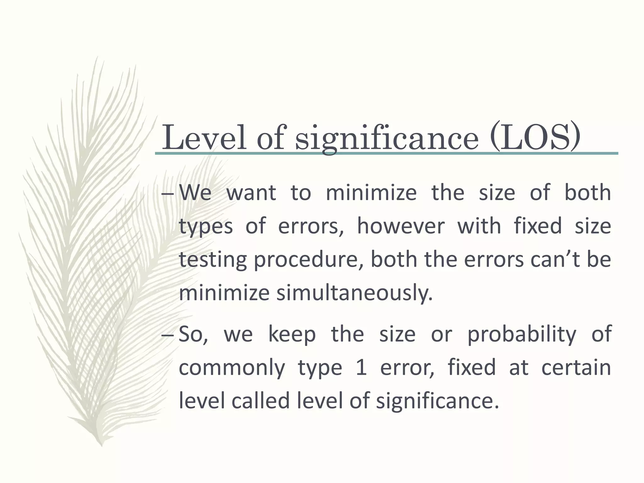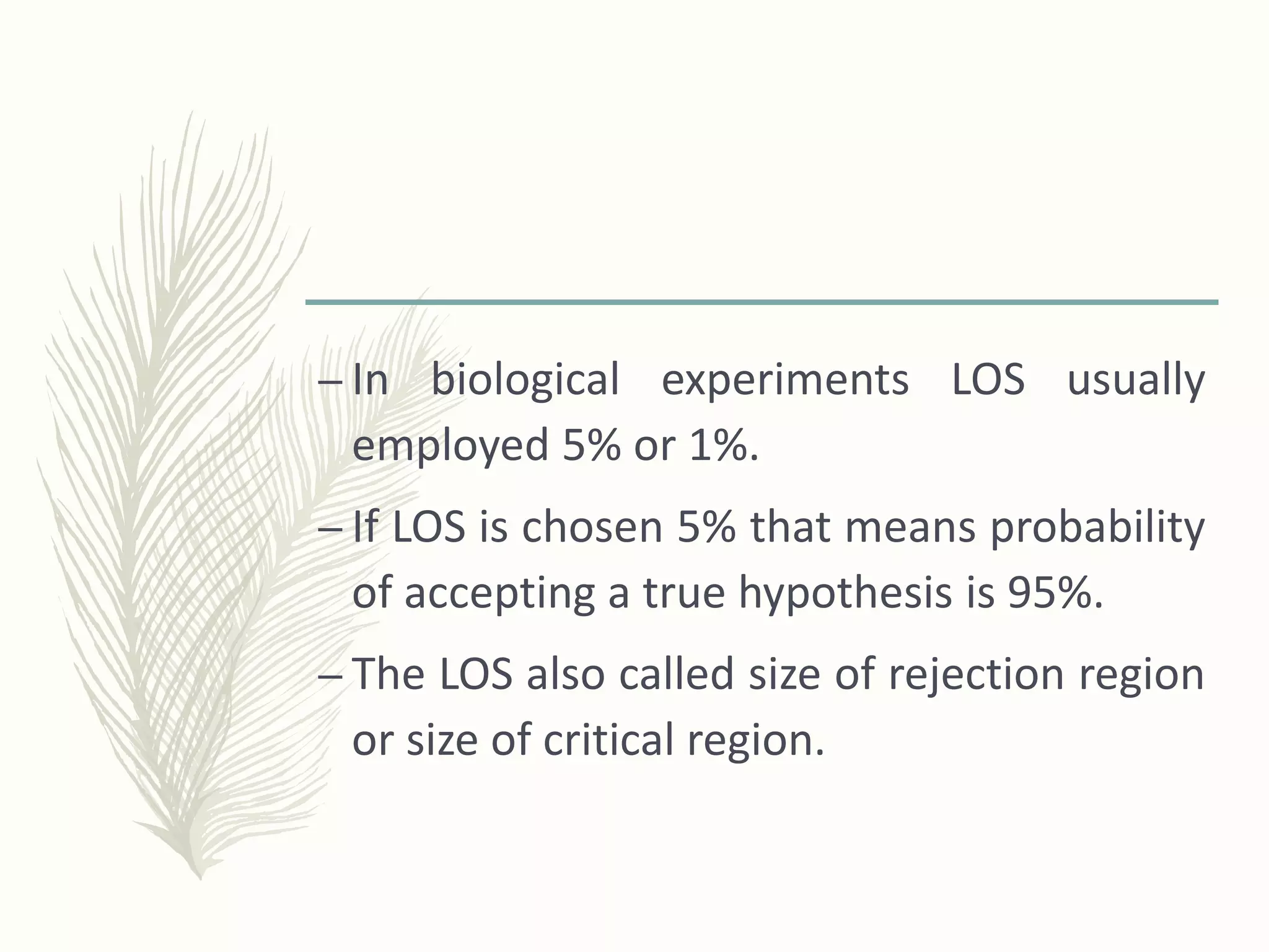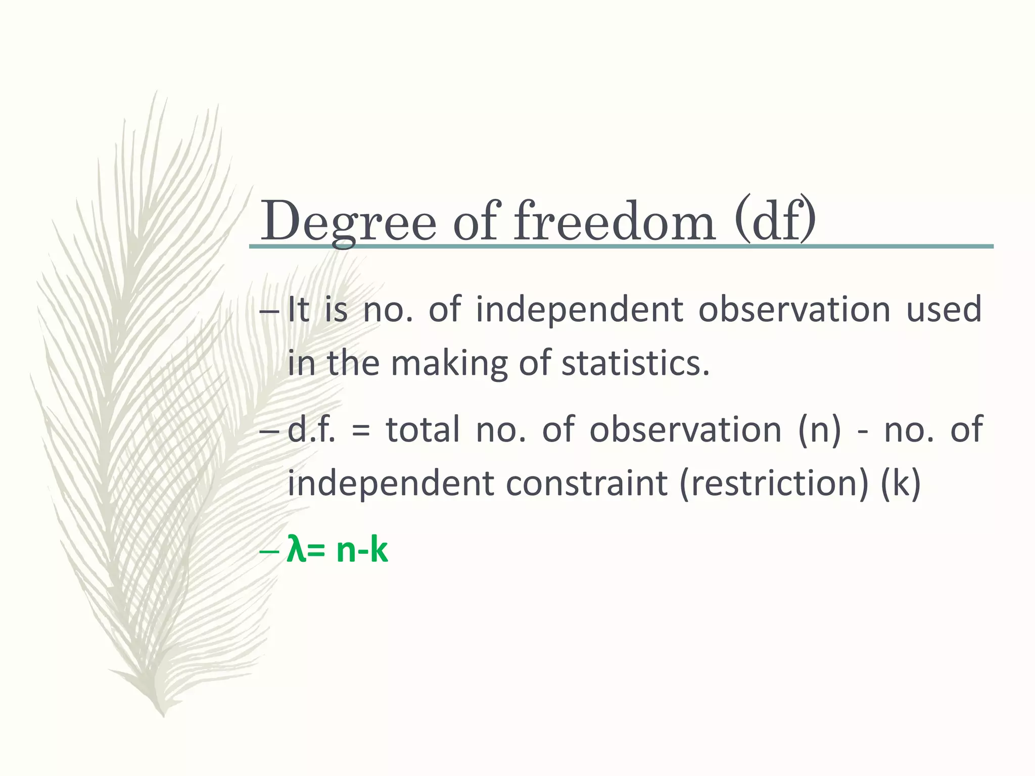The document defines key terms like null and alternative hypotheses, type I and II errors, level of significance, and degrees of freedom. It also outlines applications and procedures

1. Test of
hypothesis /
Test of
significance
Submitted by-:
Dr. Jayesh Vyas (M.V.Sc.)

2. Test of Hypothesis/ Test of
significance
– Procedure which enable us to decide
whether the accept or reject hypothesis.
– The test used to ascertain whether the
difference between estimator & parameter
or between two estimator are real or due to
chance are called test of hypothesis.

3. Terms used in testing a hypothesis
– Null hypothesis(H0)-: Hypothesis which is
tested for possible rejection, under the
assumption that is true called H0.
– Alternative hypothesis(H1)-: Hypothesis
which is complementary to null
hypothesis.

4. Type of Errors
Accept H0 Reject H0
or accept
H1
H0 is true Correct
decision
Type 1
error
H0 is false Type 2
error
Correct
decision

5. Level of significance (LOS)
– We want to minimize the size of both
types of errors, however with fixed size
testing procedure, both the errors can’t be
minimize simultaneously.
– So, we keep the size or probability of
commonly type 1 error, fixed at certain
level called level of significance.

6. – In biological experiments LOS usually
employed 5% or 1%.
– If LOS is chosen 5% that means probability
of accepting a true hypothesis is 95%.
– The LOS also called size of rejection region
or size of critical region.

7. Degree of freedom (df)
– It is no. of independent observation used
in the making of statistics.
– d.f. = total no. of observation (n) - no. of
independent constraint (restriction) (k)
– λ= n-k

8. T-test
– Developed by W. S. Gossett.
– It is parametric test.
– It is small sample test.
– Suppose 𝑥1, 𝑥2, … 𝑥 𝑛 be a random sample
size 𝑛 drawn from population with mean µ
and variance 𝜎2
, then T- statistics defined
as
– 𝐭 =
𝐗−𝛍
𝐒 𝐧
𝑋= sample mean, S= SD of sample, n= no. of observation

9. Applications of t-test
1. Test the significance of sample mean
when population variance is unknown.
𝐭 =
𝐗−𝛍
𝐒 𝐧
SD=
𝐗− 𝐗 𝟐
𝐧−𝟏
d.f. =n-1

10. 2. Testing the significance of difference between mean of 2
samples / Unpaired t- test-:2 random samples are
independent. 𝑥1, 𝑥2, … 𝑥 𝑛 be a random sample size 𝑛1 drawn
from population with mean µ1 and variance 𝜎1
2
& another
random sample 𝑦1, 𝑦2, … 𝑦𝑛 be a random sample size 𝑛2
with mean µ2 and variance 𝜎2
2
, then
𝒕 =
|𝑿− 𝒀|
𝐒
𝟏
𝒏 𝟏
+
𝟏
𝒏 𝟐
S=
X−X 2+ Y− 𝑌 2
𝑛1+𝑛2−2
d.f.=n1+n2-2 S= Pooled S.D.

11. 3. Paired t- test-: 2 random samples are dependent. (𝑥1 𝑦1),
(𝑦2 𝑥2), … (𝑥n 𝑦𝑛) be a random sample size drawn from
population n no. of pairs
t =
𝑑
S n
𝑑=
𝑑
𝑛
d=x-y
SD=
d− 𝑑 2
n−1
d.f. =n-1

12. 4. Testing the significance of correlation coefficient-:
(𝑥1 𝑦1), (𝑦2 𝑥2), … (𝑥n 𝑦𝑛) be a random sample size drawn
from bivariate population n no. of pairs then
𝒕 =
|𝒓|
𝑺.𝑬.(𝒓)
r= correlation coefficient, S.E.= Stand. Error
S.E=
𝒓 𝟐
𝒏−𝟐
d.f.=n-2

13. 5. Testing the significance of regression coefficient-: (𝑥1 𝑦1),
(𝑦2 𝑥2), … (𝑥n 𝑦 𝑛) be a random sample size drawn from bivariate
population n no. of pairs then
𝒕 =
𝒃 𝒀𝑿
𝑺.𝑬.(𝒃 𝒀𝑿)
S.E.=
𝒀− 𝒀 𝟐−𝒃 𝒀𝑿 𝑿− 𝑿 𝒀− 𝒀
𝒏−𝟐 . 𝑿− 𝑿 𝟐
d.f.=n-2

14. Chi-square (𝜒2
)- test
– It is non para-metric test.
– Easy to compute and used without making assumptions, it
is distribution free test.
– Magnitude of difference between observed & expected
frequency under certain assumption
𝝌 𝟐=
𝐎−𝑬 𝟐
𝑬
≈ 𝝌 𝟐
𝒏−𝟏 𝒅𝒇
𝑂1, 𝑂2, … 𝑂𝑛 = observed frequency
𝐸1, 𝐸2, … 𝐸 𝑛 = expected frequency

15. Applications of 𝜒2
- test
1. Testing the significance of population variance-: 𝜎0
2
is
known population variance and n is no. of sample size
𝝌 𝟐=
𝑿− 𝑿 𝟐
𝝈 𝟎
𝟐
d.f. =n-1

16. 2. Testing the goodness of fit-:
𝜒2=
𝑂−𝐸 2
𝐸
E=
𝑂
𝑛
d.f.=n-1

17. 3. Testing the independence of attribute/contingency test/test for
independence-: m rows & n columns = m*n contingency table. A
has m mutually exclusive categories 𝐴1, 𝐴2, … 𝐴 𝑚. B has n mutually
exclusive categories 𝐵1, 𝐵2, … 𝐵 𝑛.
contd...
AB 𝑩 𝟏 𝑩 𝟐 𝑩 𝒏 Total
𝐴1 AB 𝑩 𝟏 𝑩 𝟐 𝑩 𝒏 Total
𝐴1 𝑂11 𝑂12 𝑂1𝑛 𝑅1
𝐴2 𝐴2 𝑂21 𝑂22 𝑂2n 𝑅2
𝐴m 𝐴m 𝑂m1 𝑂m2 𝑂mn 𝑅m
Total Total 𝐶1 𝐶2 𝐶n N

18. C1 = sum of first column
R1 = sum of first row
N = sum of all rows
E(𝑶 𝟏𝟏)=
𝑹 𝟏 𝑪 𝟏
𝑵
, E(𝑶 𝟏𝟐)=
𝑹 𝟏 𝑪 𝟐
𝑵
, E(𝑶 𝟐𝟏)=
𝑹 𝟐 𝑪 𝟏
𝑵
E(𝑶 𝟏𝒏) = R1-[E(𝑶 𝟏𝟏)+ E(𝑶 𝟏𝟐)+…+E(𝑶 𝐧−𝟏)]
E(𝑶 𝐦𝟏) = C1-[E(𝑶 𝟏𝟏)+ E(𝑶 𝟐𝟏)+…+E(𝑶 𝐦−𝟏)]
d.f. = (row-1)(column-1) contd…

19. O E O-E 𝑶 − 𝑬 𝟐 𝐎 − 𝑬 𝟐
𝑬
𝑂11 E(𝑂11)
𝑂12 E(𝑂12)
𝑂mn E(𝑂mn) Total (Value of
𝜒2
)

20. 4. Testing the independence of attribute in contingency table-:
Only 2 categories = 2 rows*2 columns then
Contd….
AB 𝑩 𝟏 𝑩 𝟐 Total
𝐴1 𝑂11(a) 𝑂12(b) 𝑅1
𝐴2 𝑂21(c) 𝑂12(d) 𝑅2
C1 C2 N

21. 𝜒2=
𝐚𝐝−𝒃𝒄 𝟐 𝑵
𝑅1 𝑅2 𝐶1 𝐶2
d.f. = (row-1)(column-1)
d.f. = 1 always
 If any observed cell frequency is <5 then we used Yate’s
correction
 𝝌 𝟐
=
|𝐚𝐝−𝒃𝒄|−
𝑵
𝟐
𝟐
𝑵
𝑹 𝟏 𝑹 𝟐 𝑪 𝟏 𝑪 𝟐

22. F-Test
– The object of F-test is to find out whether the 2
independent estimates of population variance differs
significantly.
– It is a parametric test.
– There are 2 degree of freedoms.
𝐹1 =
𝑺 𝟏
𝟐
𝑺 𝟐
𝟐 , 𝑺 𝟏
𝟐
=
𝑿− 𝑿 𝟐
𝒏 𝟏−𝟏
, 𝑺 𝟐
𝟐
=
𝒀− 𝒀 𝟐
𝒏 𝟐−𝟏

23. Applications of F- test
1. Testing of significance of ratio of 2 variances-:
𝐹1 =
𝑺 𝟏
𝟐
𝑺 𝟐
𝟐
d.f. = n1-1 for numerator
d.f. = n2-2 for denominator

24. 2. Testing the homogeneity of several means-: Significance
of difference amongst more than 2 sample means is
carried out at the same time and this technique is
known as analysis of variance (ANOVA).
Contd…

25. ANOVA
– When observations are classified on the basis of single
criteria from K random samples.
Sample no. Total
1 𝑌11 𝑌12 𝑌1𝑛1
𝑇1
2 𝑌21 𝑌22 𝑌2𝑛2
𝑇2
𝑘 𝑌𝑘𝑛1
𝑌𝑘𝑛2
𝑌𝑘𝑛 𝑘
𝑇k
Total G

26. – Correction factor C.F.=
𝐺2
𝑛
, G= Grand total n = n.k
– Total sum of sum of square TSS
– TSS = 𝛴𝑌ⅈ𝑗
2
− 𝐶. 𝐹. , 𝛴𝑌ⅈ𝑗
2
= Sum of square
– Sum of square due to assignable factor S.S.assign
– S.S.assign = (
𝑇1
2
𝑛1
+
𝑇2
2
𝑛2
+…+
𝑇𝑘
2
𝑛k
)- C.F.
– Sum of square due to non assignable factor S.S.Error
– S.S.Error= TSS- S.S.assign

27. – Preparation of ANOVA Table-:
– d.f.= k-1 for numerator & n-k for denominator
Source of
variation
d.f. S.S. M.S.S. F-value
B/t assign 𝑘 − 1 S1
𝑠1
𝑘−1
= V1
𝑉1
𝑉2
= F-value
Error 𝑛 − 𝑘 S2
𝑠1
𝑘−1
=V2
Total 𝑛 − 1 S