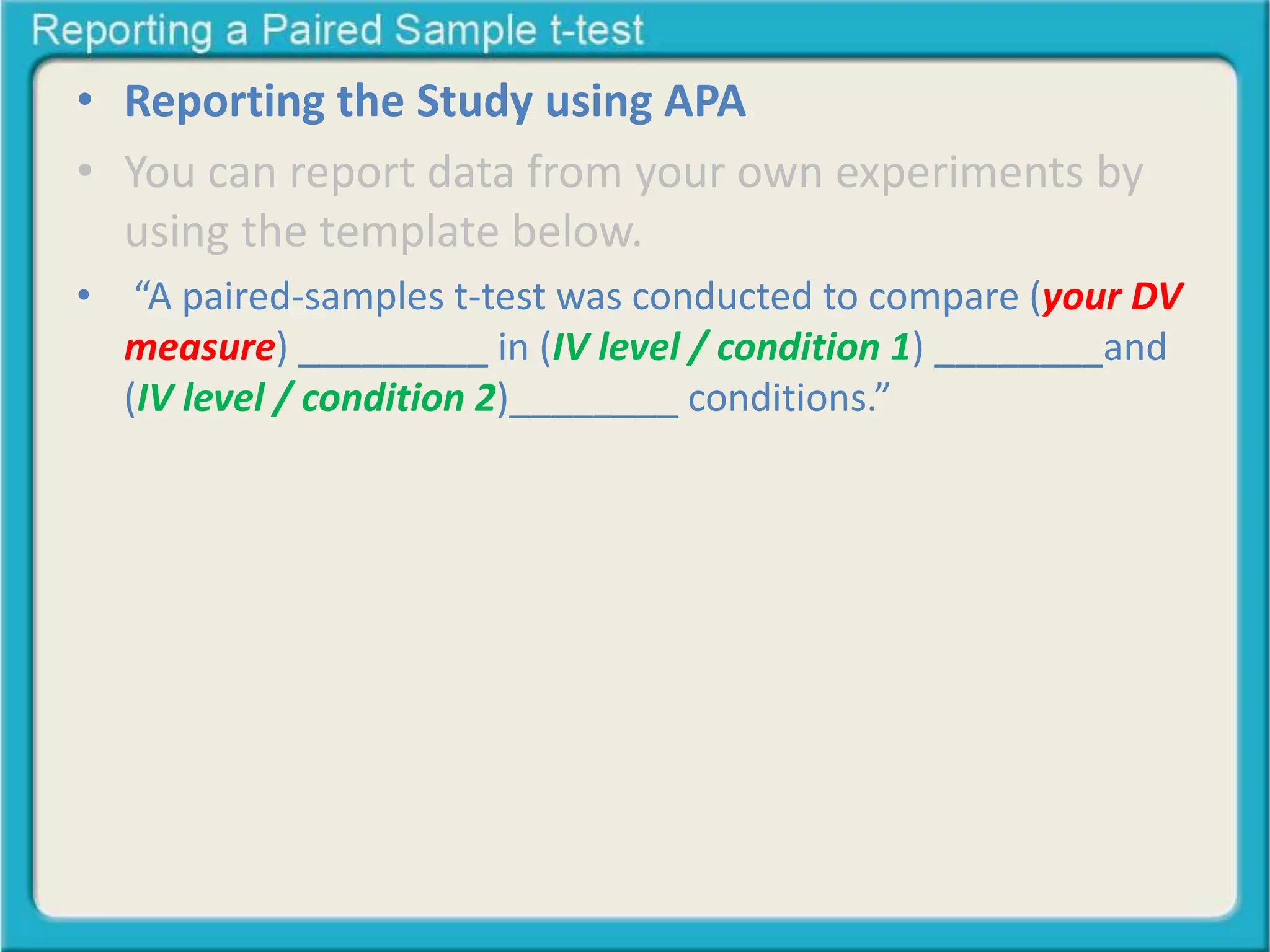
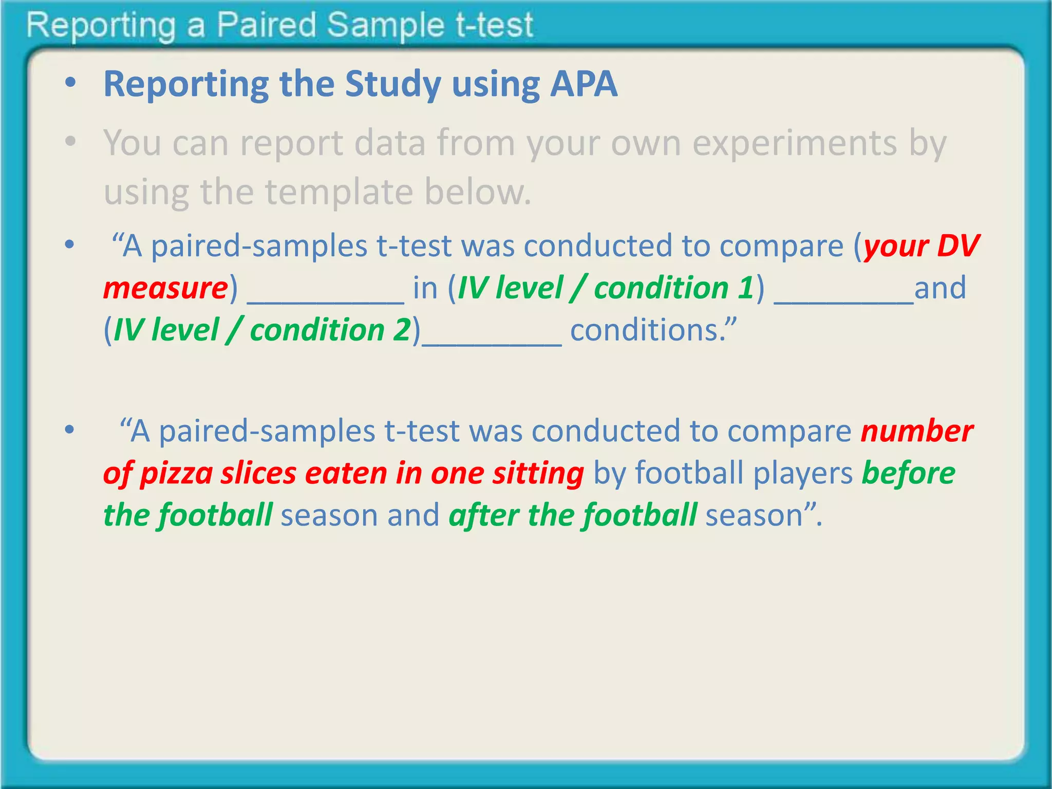
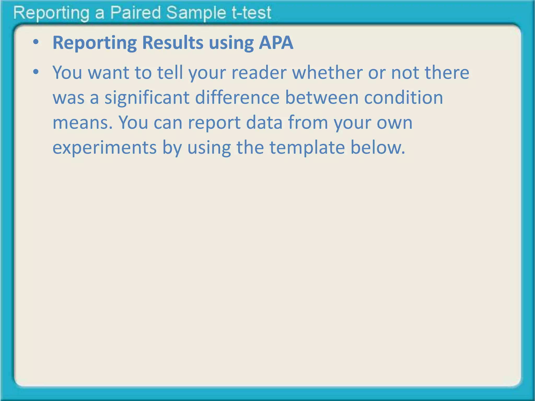
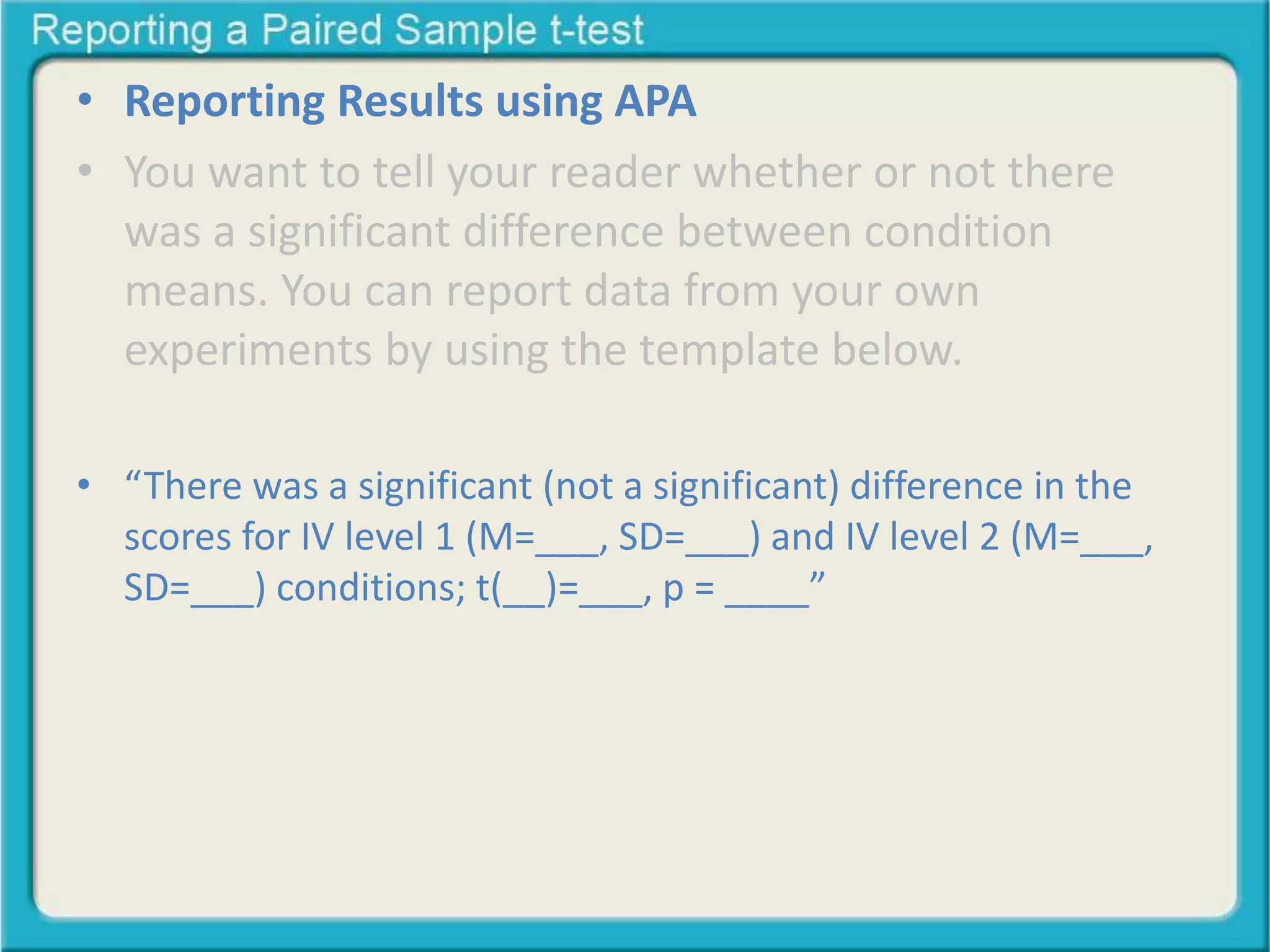
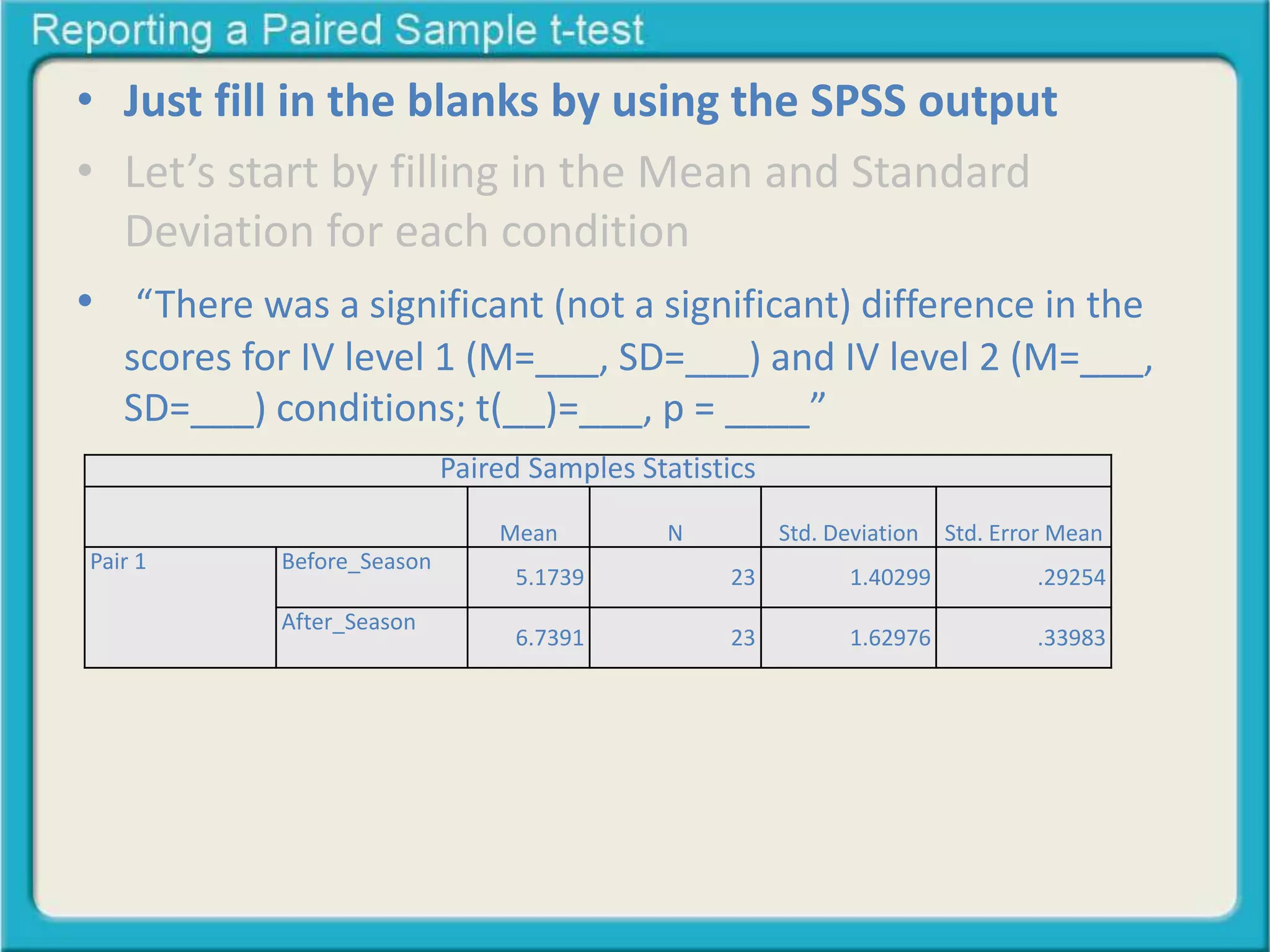
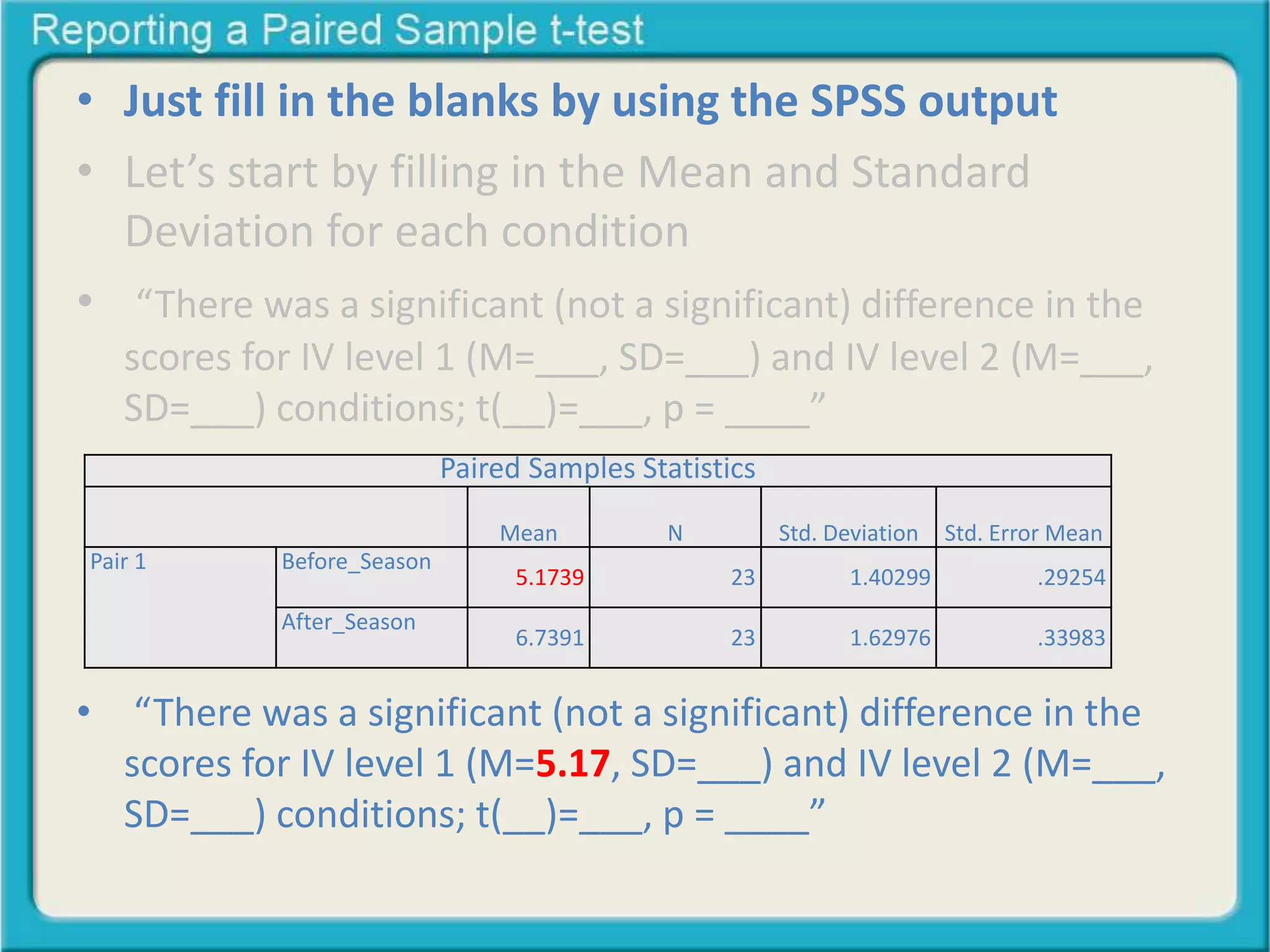
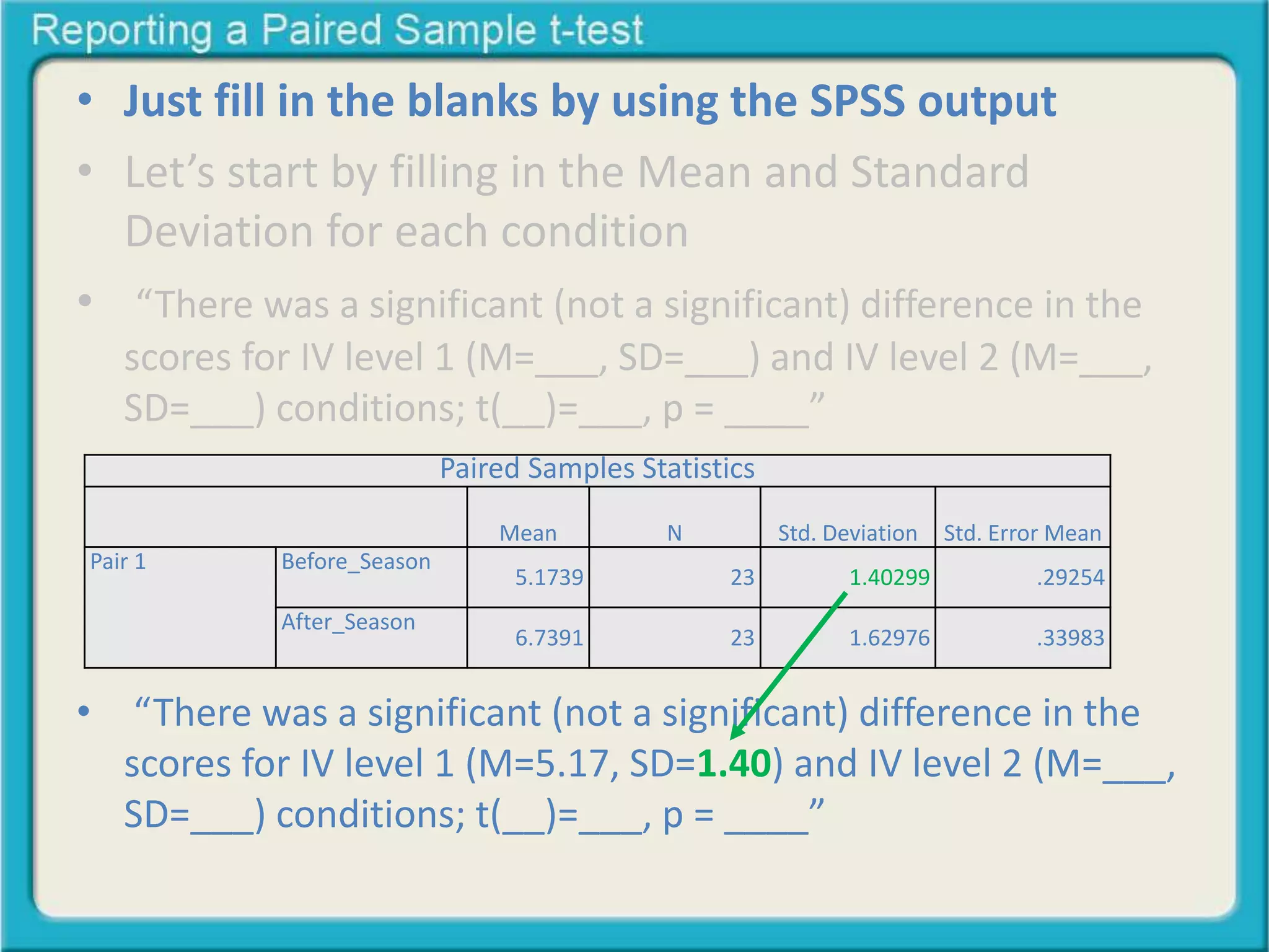
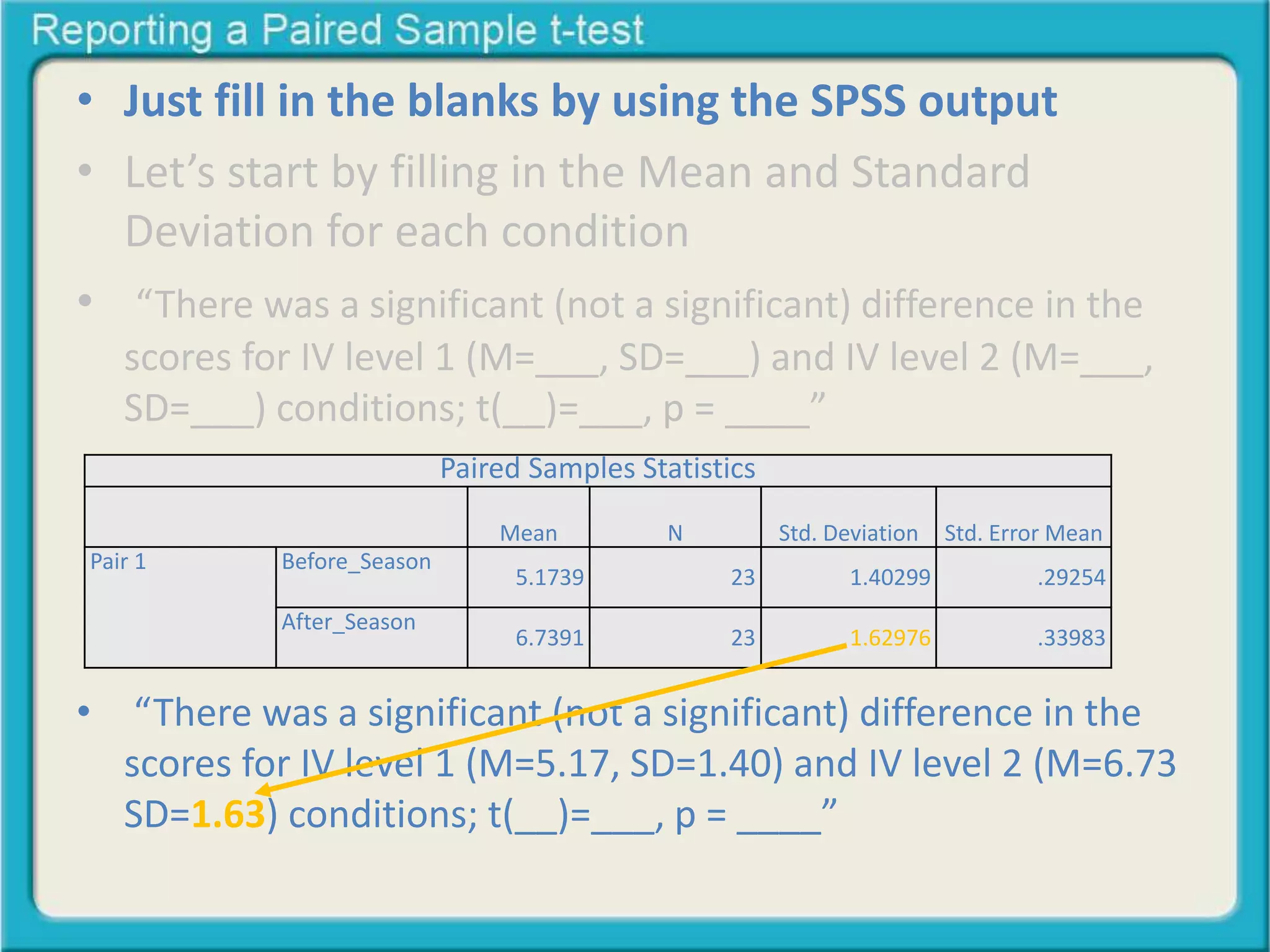
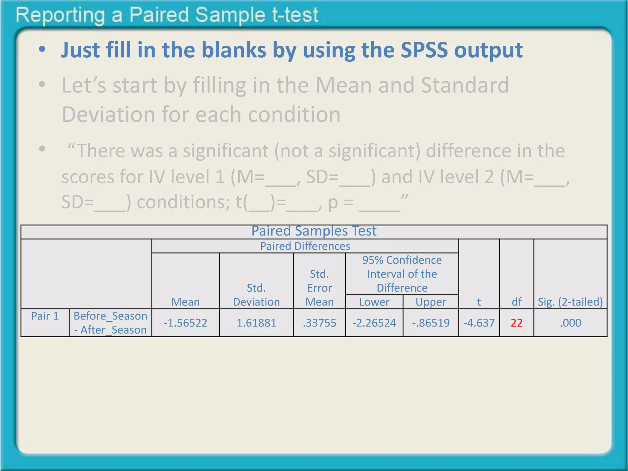
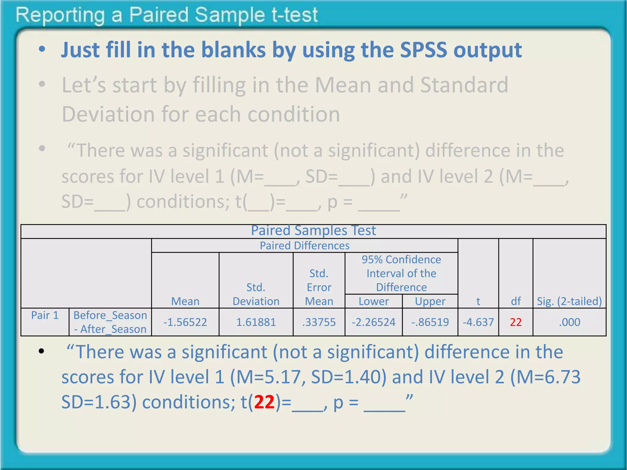
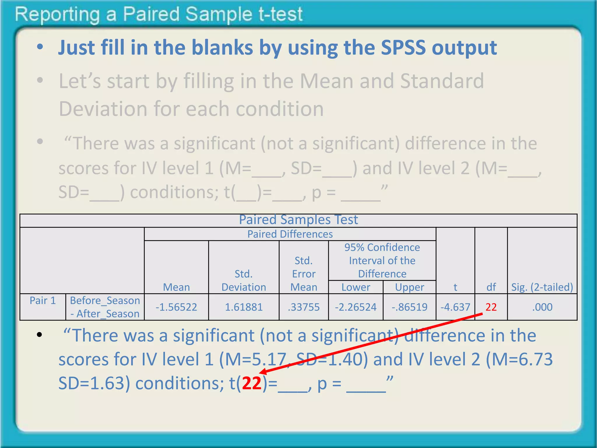
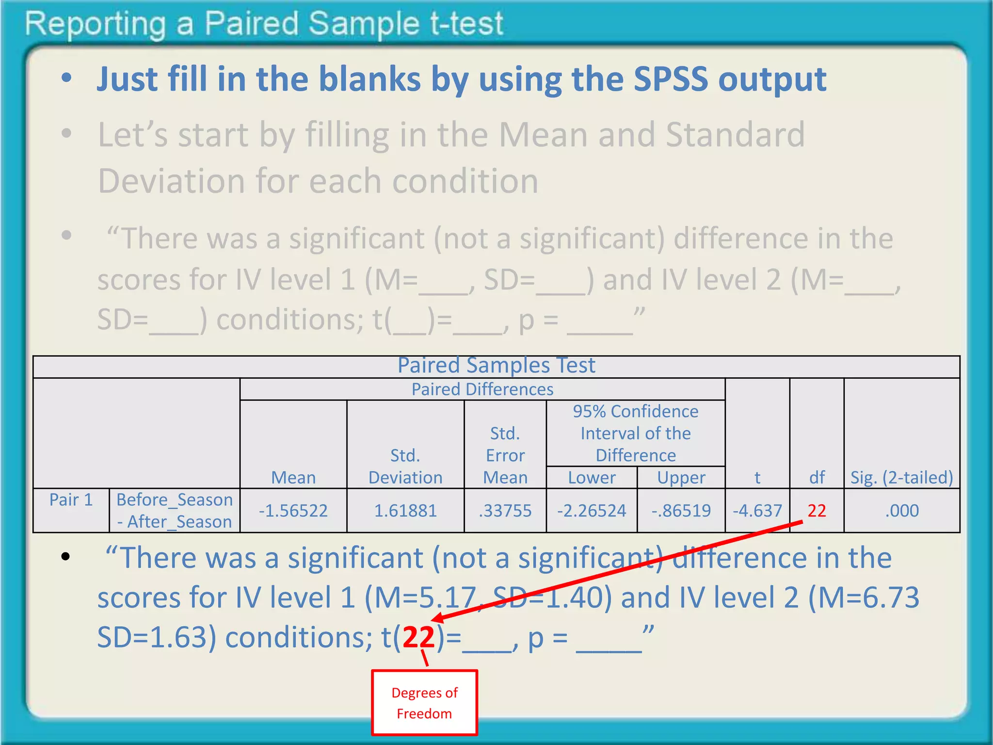
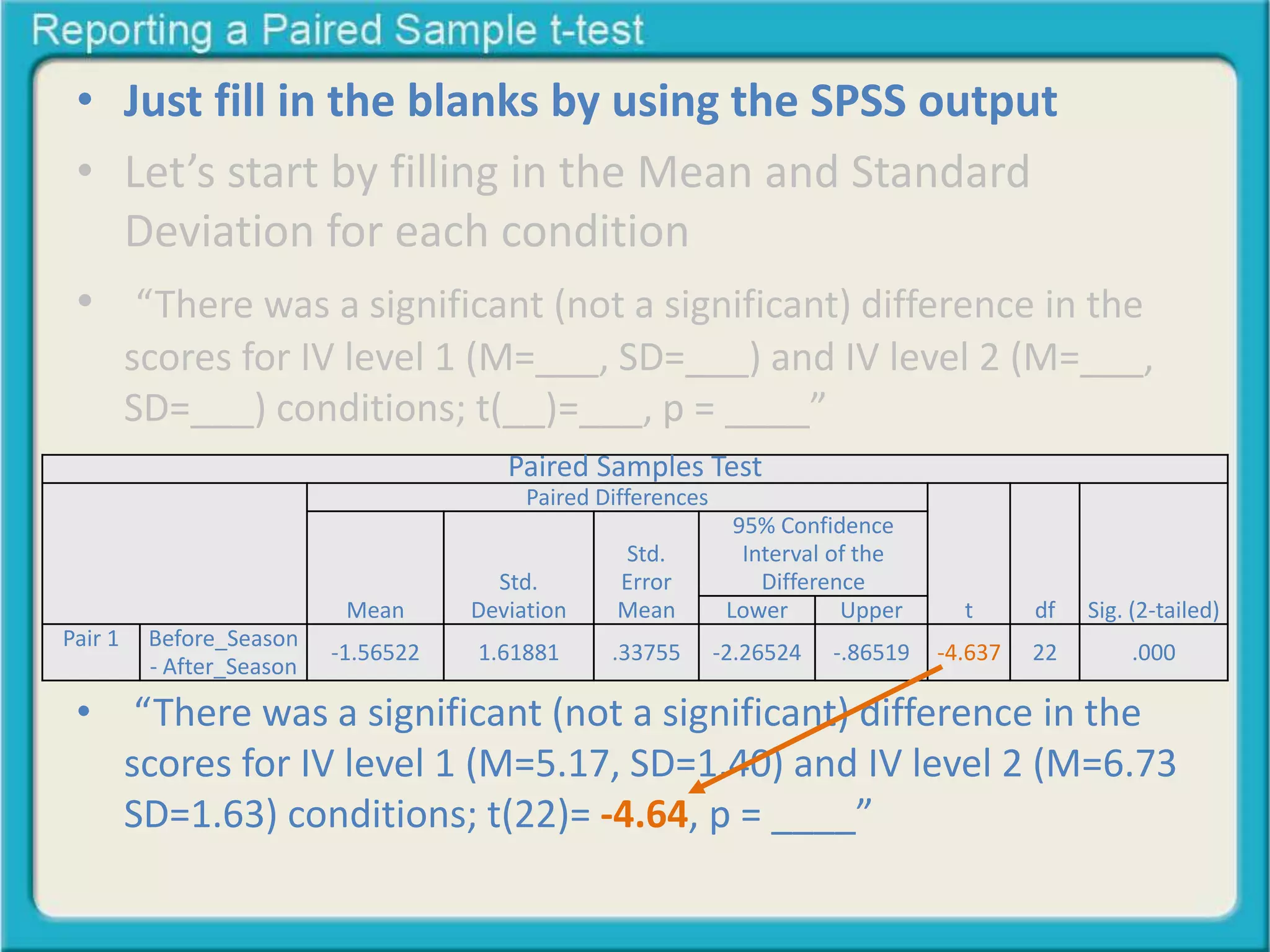
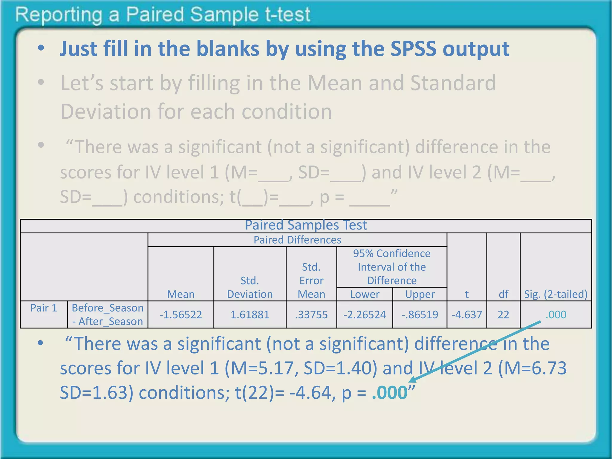
The document provides guidance on reporting the results of a paired sample t-test in APA format. It includes templates for reporting the study design, results, and statistical analysis. Key details include reporting the means, standard deviations, and standard errors for each condition. It also notes reporting the t-statistic, degrees of freedom, and significance level based on the t-test output.

1. Reporting a Paired Sample t-test

2. Reporting a Paired Sample t-test
Note – that the reporting format shown
in this learning module is for APA. For
other formats consult specific format
guides.

3. Reporting a Paired Sample t-test
Note – that the reporting format shown
in this learning module is for APA. For
other formats consult specific format
guides.
It is also recommended to consult the
latest APA manual to compare what is
described in this learning module with
the most updated formats for APA.

4. • Reporting the Study using APA

5. • Reporting the Study using APA
• You can report data from your own experiments by
using the template below.

6. • Reporting the Study using APA
• You can report data from your own experiments by
using the template below.
• “A paired-samples t-test was conducted to compare (your DV
measure) _________ in (IV level / condition 1) ________and
(IV level / condition 2)________ conditions.”

7. • Reporting the Study using APA
• You can report data from your own experiments by
using the template below.
• “A paired-samples t-test was conducted to compare (your DV
measure) _________ in (IV level / condition 1) ________and
(IV level / condition 2)________ conditions.”
• “A paired-samples t-test was conducted to compare number
of pizza slices eaten in one sitting by football players before
the football season and after the football season”.

8. • Reporting Results using APA

9. • Reporting Results using APA
• You want to tell your reader whether or not there
was a significant difference between condition
means. You can report data from your own
experiments by using the template below.

10. • Reporting Results using APA
• You want to tell your reader whether or not there
was a significant difference between condition
means. You can report data from your own
experiments by using the template below.
• “There was a significant (not a significant) difference in the
scores for IV level 1 (M=___, SD=___) and IV level 2 (M=___,
SD=___) conditions; t(__)=___, p = ____”

11. • Just fill in the blanks by using the SPSS output

12. • Just fill in the blanks by using the SPSS output
• Let’s start by filling in the Mean and Standard
Deviation for each condition

13. • Just fill in the blanks by using the SPSS output
• Let’s start by filling in the Mean and Standard
Deviation for each condition
• “There was a significant (not a significant) difference in the
scores for IV level 1 (M=___, SD=___) and IV level 2 (M=___,
SD=___) conditions; t(__)=___, p = ____”

14. • Just fill in the blanks by using the SPSS output
• Let’s start by filling in the Mean and Standard
Deviation for each condition
• “There was a significant (not a significant) difference in the
scores for IV level 1 (M=___, SD=___) and IV level 2 (M=___,
SD=___) conditions; t(__)=___, p = ____”
Paired Samples Statistics
Mean N Std. Deviation Std. Error Mean
Pair 1 Before_Season
5.1739 23 1.40299 .29254
After_Season
6.7391 23 1.62976 .33983

15. • Just fill in the blanks by using the SPSS output
• Let’s start by filling in the Mean and Standard
Deviation for each condition
• “There was a significant (not a significant) difference in the
scores for IV level 1 (M=___, SD=___) and IV level 2 (M=___,
SD=___) conditions; t(__)=___, p = ____”
Paired Samples Statistics
Mean N Std. Deviation Std. Error Mean
Pair 1 Before_Season
5.1739 23 1.40299 .29254
After_Season
6.7391 23 1.62976 .33983
• “There was a significant (not a significant) difference in the
scores for IV level 1 (M=5.17, SD=___) and IV level 2 (M=___,
SD=___) conditions; t(__)=___, p = ____”

16. • Just fill in the blanks by using the SPSS output
• Let’s start by filling in the Mean and Standard
Deviation for each condition
• “There was a significant (not a significant) difference in the
scores for IV level 1 (M=___, SD=___) and IV level 2 (M=___,
SD=___) conditions; t(__)=___, p = ____”
Paired Samples Statistics
Mean N Std. Deviation Std. Error Mean
Pair 1 Before_Season
5.1739 23 1.40299 .29254
After_Season
6.7391 23 1.62976 .33983
• “There was a significant (not a significant) difference in the
scores for IV level 1 (M=5.17, SD=___) and IV level 2 (M=___,
SD=___) conditions; t(__)=___, p = ____”

17. • Just fill in the blanks by using the SPSS output
• Let’s start by filling in the Mean and Standard
Deviation for each condition
• “There was a significant (not a significant) difference in the
scores for IV level 1 (M=___, SD=___) and IV level 2 (M=___,
SD=___) conditions; t(__)=___, p = ____”
Paired Samples Statistics
Mean N Std. Deviation Std. Error Mean
Pair 1 Before_Season
5.1739 23 1.40299 .29254
After_Season
6.7391 23 1.62976 .33983
• “There was a significant (not a significant) difference in the
scores for IV level 1 (M=5.17, SD=1.40) and IV level 2 (M=___,
SD=___) conditions; t(__)=___, p = ____”

18. • Just fill in the blanks by using the SPSS output
• Let’s start by filling in the Mean and Standard
Deviation for each condition
• “There was a significant (not a significant) difference in the
scores for IV level 1 (M=___, SD=___) and IV level 2 (M=___,
SD=___) conditions; t(__)=___, p = ____”
Paired Samples Statistics
Mean N Std. Deviation Std. Error Mean
Pair 1 Before_Season
5.1739 23 1.40299 .29254
After_Season
6.7391 23 1.62976 .33983
• “There was a significant (not a significant) difference in the
scores for IV level 1 (M=5.17, SD=1.40) and IV level 2 (M=___,
SD=___) conditions; t(__)=___, p = ____”

19. • Just fill in the blanks by using the SPSS output
• Let’s start by filling in the Mean and Standard
Deviation for each condition
• “There was a significant (not a significant) difference in the
scores for IV level 1 (M=___, SD=___) and IV level 2 (M=___,
SD=___) conditions; t(__)=___, p = ____”
Paired Samples Statistics
Mean N Std. Deviation Std. Error Mean
Pair 1 Before_Season
5.1739 23 1.40299 .29254
After_Season
6.7391 23 1.62976 .33983
• “There was a significant (not a significant) difference in the
scores for IV level 1 (M=5.17, SD=1.40) and IV level 2 (M=6.73
SD=___) conditions; t(__)=___, p = ____”

20. • Just fill in the blanks by using the SPSS output
• Let’s start by filling in the Mean and Standard
Deviation for each condition
• “There was a significant (not a significant) difference in the
scores for IV level 1 (M=___, SD=___) and IV level 2 (M=___,
SD=___) conditions; t(__)=___, p = ____”
Paired Samples Statistics
Mean N Std. Deviation Std. Error Mean
Pair 1 Before_Season
5.1739 23 1.40299 .29254
After_Season
6.7391 23 1.62976 .33983
• “There was a significant (not a significant) difference in the
scores for IV level 1 (M=5.17, SD=1.40) and IV level 2 (M=6.73
SD=___) conditions; t(__)=___, p = ____”

21. • Just fill in the blanks by using the SPSS output
• Let’s start by filling in the Mean and Standard
Deviation for each condition
• “There was a significant (not a significant) difference in the
scores for IV level 1 (M=___, SD=___) and IV level 2 (M=___,
SD=___) conditions; t(__)=___, p = ____”
Paired Samples Statistics
Mean N Std. Deviation Std. Error Mean
Pair 1 Before_Season
5.1739 23 1.40299 .29254
After_Season
6.7391 23 1.62976 .33983
• “There was a significant (not a significant) difference in the
scores for IV level 1 (M=5.17, SD=1.40) and IV level 2 (M=6.73
SD=1.63) conditions; t(__)=___, p = ____”

22. • Just fill in the blanks by using the SPSS output
• Let’s start by filling in the Mean and Standard
Deviation for each condition
• “There was a significant (not a significant) difference in the
scores for IV level 1 (M=___, SD=___) and IV level 2 (M=___,
SD=___) conditions; t(__)=___, p = ____”
Paired Samples Statistics
Mean N Std. Deviation Std. Error Mean
Pair 1 Before_Season
5.1739 23 1.40299 .29254
After_Season
6.7391 23 1.62976 .33983
• “There was a significant (not a significant) difference in the
scores for IV level 1 (M=5.17, SD=1.40) and IV level 2 (M=6.73
SD=1.63) conditions; t(__)=___, p = ____”

23. • Just fill in the blanks by using the SPSS output
• Let’s start by filling in the Mean and Standard
Deviation for each condition
• “There was a significant (not a significant) difference in the
scores for IV level 1 (M=___, SD=___) and IV level 2 (M=___,
SD=___) conditions; t(__)=___, p = ____”
Paired Samples Test
Paired Differences
Std.
Deviation
Std.
Error
Mean
95% Confidence
Interval of the
Difference
Mean Lower Upper
t df Sig. (2-tailed)
Pair 1 Before_Season
- After_Season
-1.56522 1.61881 .33755 -2.26524 -.86519 -4.637 22 .000

24. • Just fill in the blanks by using the SPSS output
• Let’s start by filling in the Mean and Standard
Deviation for each condition
• “There was a significant (not a significant) difference in the
scores for IV level 1 (M=___, SD=___) and IV level 2 (M=___,
SD=___) conditions; t(__)=___, p = ____”
Paired Samples Test
Paired Differences
Std.
Deviation
Std.
Error
Mean
95% Confidence
Interval of the
Difference
Mean Lower Upper
t df Sig. (2-tailed)
Pair 1 Before_Season
- After_Season
-1.56522 1.61881 .33755 -2.26524 -.86519 -4.637 22 .000
• “There was a significant (not a significant) difference in the
scores for IV level 1 (M=5.17, SD=1.40) and IV level 2 (M=6.73
SD=1.63) conditions; t(22)=___, p = ____”

25. • Just fill in the blanks by using the SPSS output
• Let’s start by filling in the Mean and Standard
Deviation for each condition
• “There was a significant (not a significant) difference in the
scores for IV level 1 (M=___, SD=___) and IV level 2 (M=___,
SD=___) conditions; t(__)=___, p = ____”
Paired Samples Test
Paired Differences
Std.
Deviation
Std.
Error
Mean
95% Confidence
Interval of the
Difference
Mean Lower Upper
t df Sig. (2-tailed)
Pair 1 Before_Season
- After_Season
-1.56522 1.61881 .33755 -2.26524 -.86519 -4.637 22 .000
• “There was a significant (not a significant) difference in the
scores for IV level 1 (M=5.17, SD=1.40) and IV level 2 (M=6.73
SD=1.63) conditions; t(22)=___, p = ____”

26. • Just fill in the blanks by using the SPSS output
• Let’s start by filling in the Mean and Standard
Deviation for each condition
• “There was a significant (not a significant) difference in the
scores for IV level 1 (M=___, SD=___) and IV level 2 (M=___,
SD=___) conditions; t(__)=___, p = ____”
Paired Samples Test
Paired Differences
Std.
Deviation
Std.
Error
Mean
95% Confidence
Interval of the
Difference
Mean Lower Upper
t df Sig. (2-tailed)
Pair 1 Before_Season
- After_Season
-1.56522 1.61881 .33755 -2.26524 -.86519 -4.637 22 .000
• “There was a significant (not a significant) difference in the
scores for IV level 1 (M=5.17, SD=1.40) and IV level 2 (M=6.73
SD=1.63) conditions; t(22)=___, p = ____”
Degrees of
Freedom

27. • Just fill in the blanks by using the SPSS output
• Let’s start by filling in the Mean and Standard
Deviation for each condition
• “There was a significant (not a significant) difference in the
scores for IV level 1 (M=___, SD=___) and IV level 2 (M=___,
SD=___) conditions; t(__)=___, p = ____”
Paired Samples Test
Paired Differences
Std.
Deviation
Std.
Error
Mean
95% Confidence
Interval of the
Difference
Mean Lower Upper
t df Sig. (2-tailed)
Pair 1 Before_Season
- After_Season
-1.56522 1.61881 .33755 -2.26524 -.86519 -4.637 22 .000
• “There was a significant (not a significant) difference in the
scores for IV level 1 (M=5.17, SD=1.40) and IV level 2 (M=6.73
SD=1.63) conditions; t(22)= -4.64, p = ____”

28. • Just fill in the blanks by using the SPSS output
• Let’s start by filling in the Mean and Standard
Deviation for each condition
• “There was a significant (not a significant) difference in the
scores for IV level 1 (M=___, SD=___) and IV level 2 (M=___,
SD=___) conditions; t(__)=___, p = ____”
Paired Samples Test
Paired Differences
Std.
Deviation
Std.
Error
Mean
95% Confidence
Interval of the
Difference
Mean Lower Upper
t df Sig. (2-tailed)
Pair 1 Before_Season
- After_Season
-1.56522 1.61881 .33755 -2.26524 -.86519 -4.637 22 .000
• “There was a significant (not a significant) difference in the
scores for IV level 1 (M=5.17, SD=1.40) and IV level 2 (M=6.73
SD=1.63) conditions; t(22)= -4.64, p = ____”

29. • Just fill in the blanks by using the SPSS output
• Let’s start by filling in the Mean and Standard
Deviation for each condition
• “There was a significant (not a significant) difference in the
scores for IV level 1 (M=___, SD=___) and IV level 2 (M=___,
SD=___) conditions; t(__)=___, p = ____”
Paired Samples Test
Paired Differences
Std.
Deviation
Std.
Error
Mean
95% Confidence
Interval of the
Difference
Mean Lower Upper
t df Sig. (2-tailed)
Pair 1 Before_Season
- After_Season
-1.56522 1.61881 .33755 -2.26524 -.86519 -4.637 22 .000
• “There was a significant (not a significant) difference in the
scores for IV level 1 (M=5.17, SD=1.40) and IV level 2 (M=6.73
SD=1.63) conditions; t(22)= -4.64, p = .000”

30. • Just fill in the blanks by using the SPSS output
• Let’s start by filling in the Mean and Standard
Deviation for each condition
• “There was a significant (not a significant) difference in the
scores for IV level 1 (M=___, SD=___) and IV level 2 (M=___,
SD=___) conditions; t(__)=___, p = ____”
Paired Samples Test
Paired Differences
Std.
Deviation
Std.
Error
Mean
95% Confidence
Interval of the
Difference
Mean Lower Upper
t df Sig. (2-tailed)
Pair 1 Before_Season
- After_Season
-1.56522 1.61881 .33755 -2.26524 -.86519 -4.637 22 .000
• “There was a significant (not a significant) difference in the
scores for IV level 1 (M=5.17, SD=1.40) and IV level 2 (M=6.73
SD=1.63) conditions; t(22)= -4.64, p = .000”

31. Here the final result:

32. “There was a significant increase in the number of
pizza slices eaten by football players after the season
(M=5.17, SD=1.40) than before the season (M=6.73
SD=1.63); t(22)= 4.64, p = .000”