Downloaded 376 times
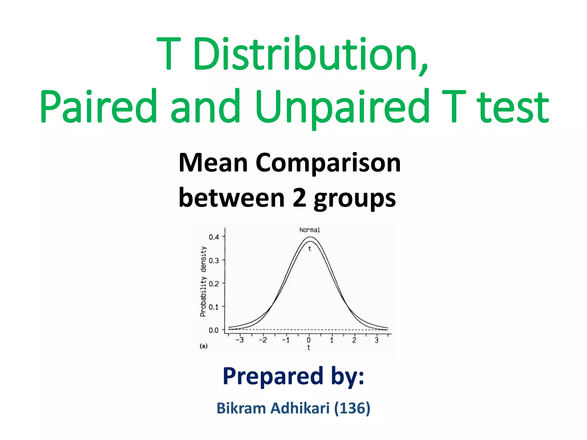
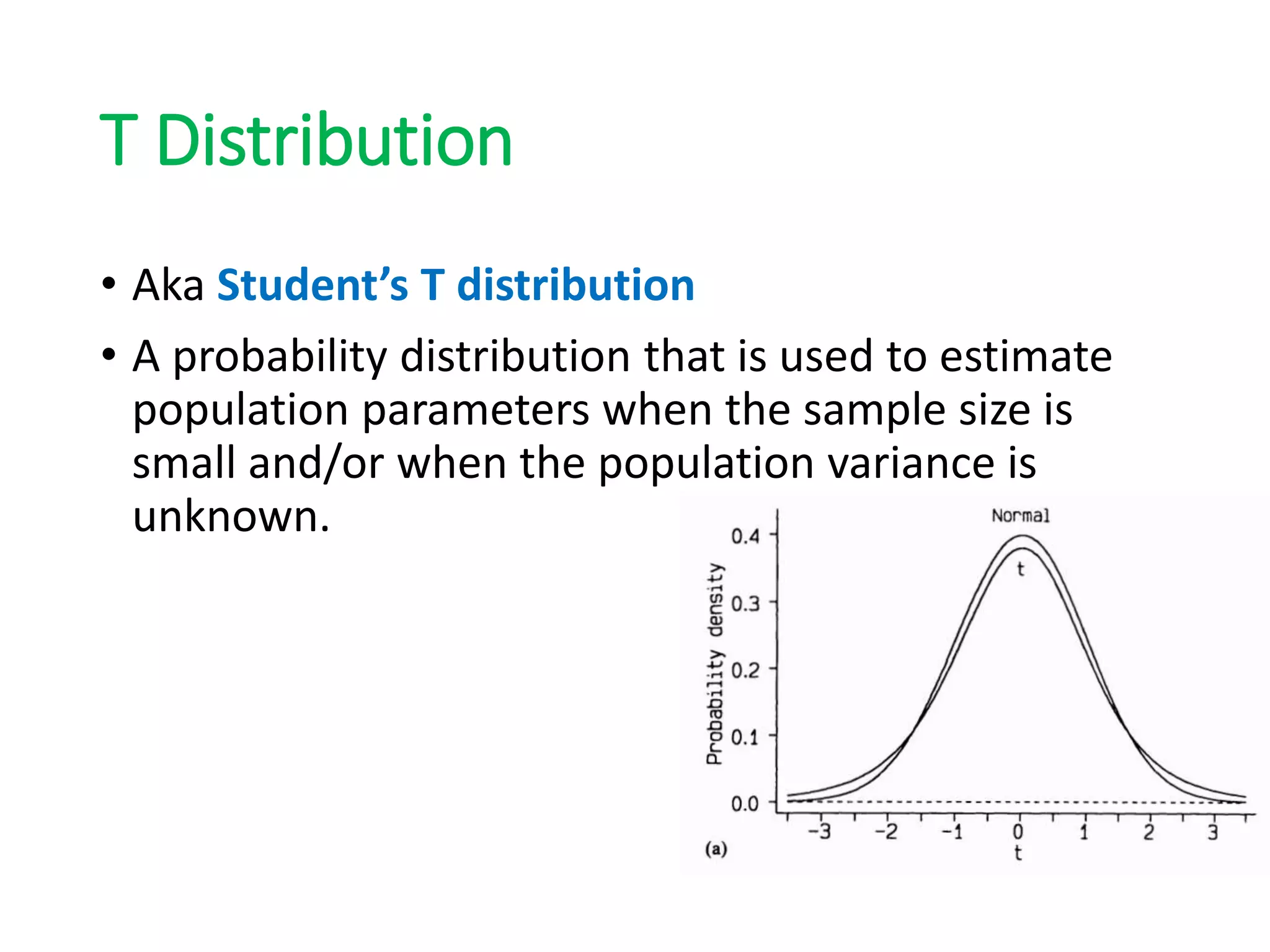
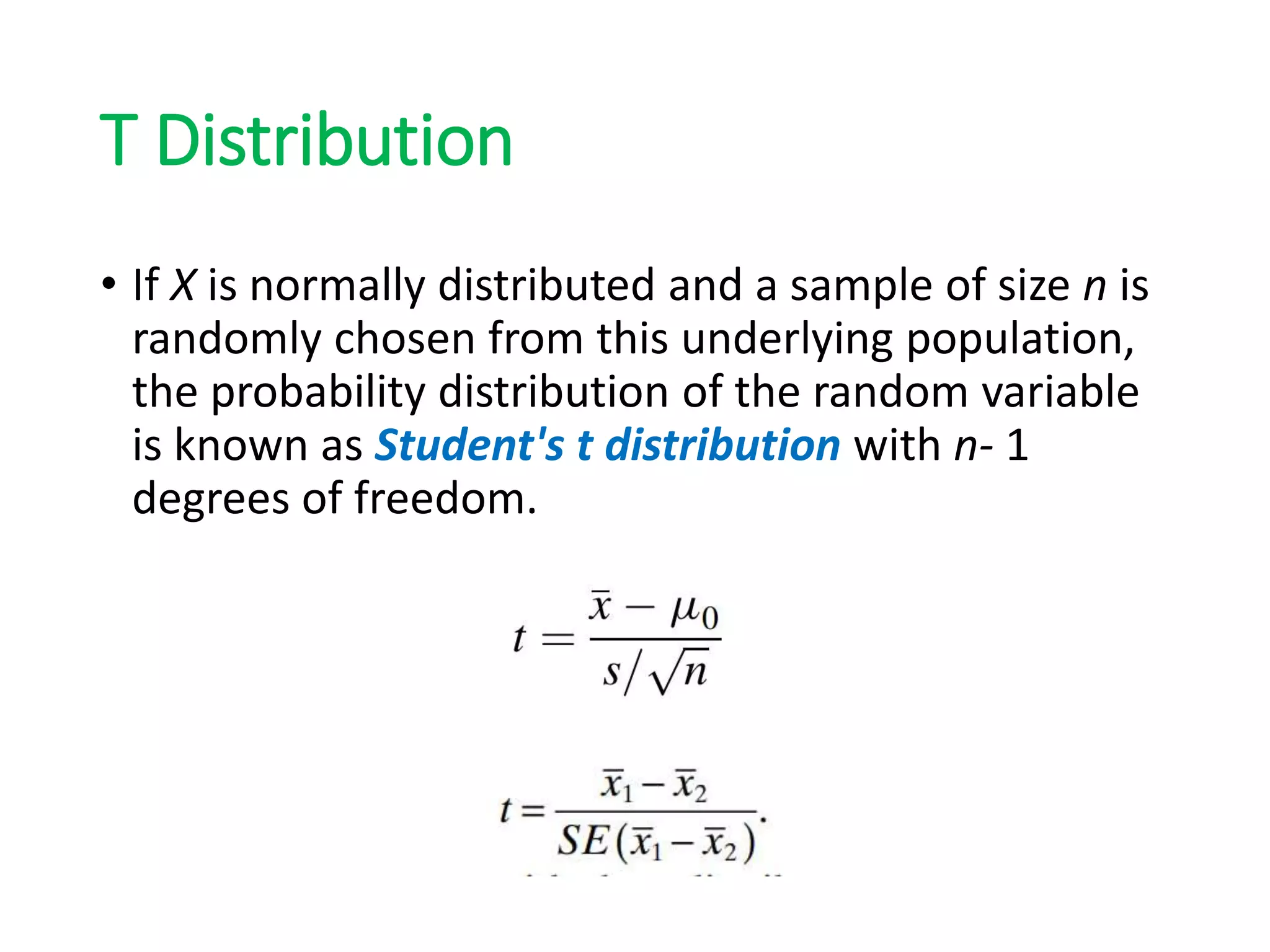
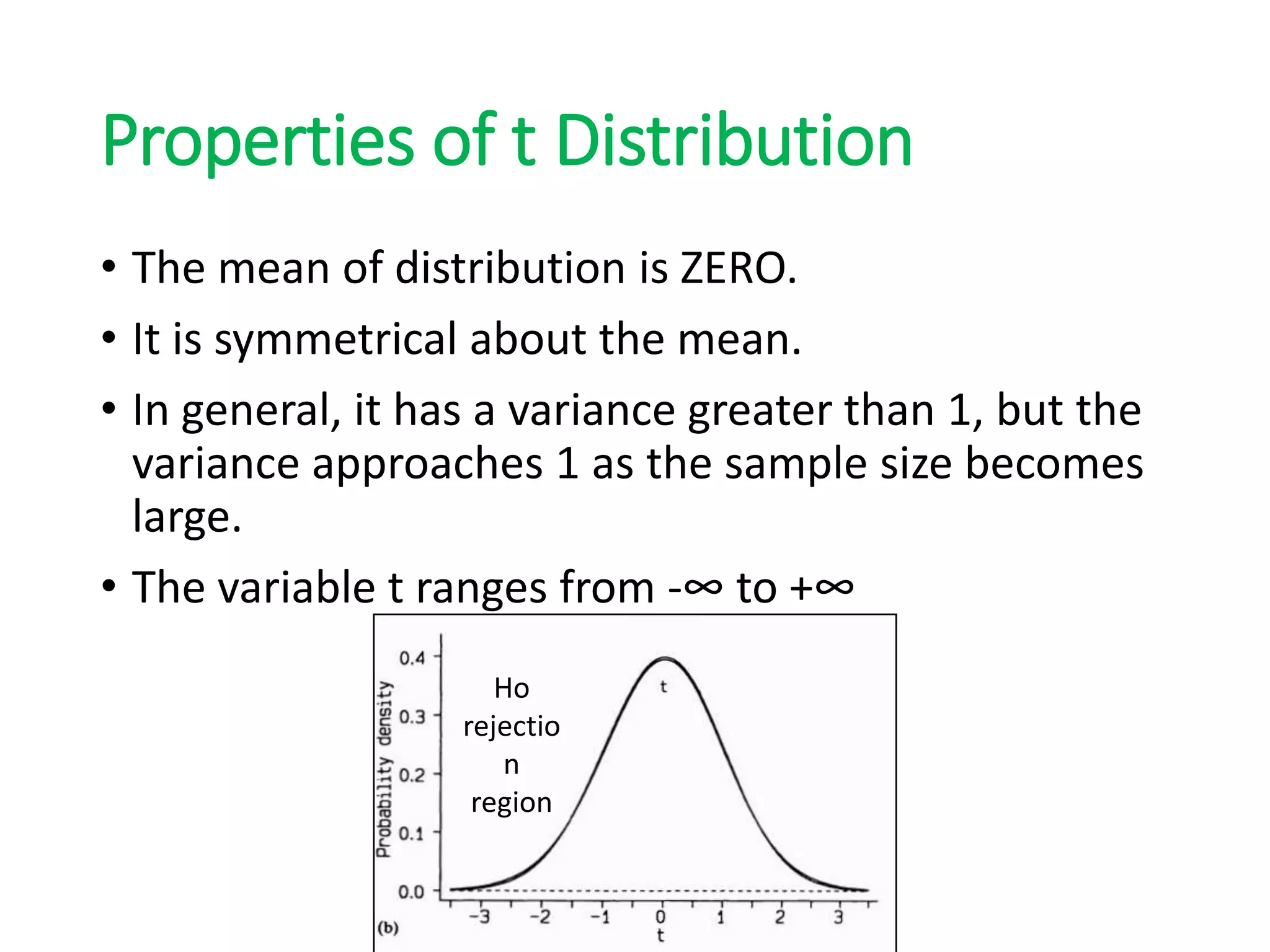

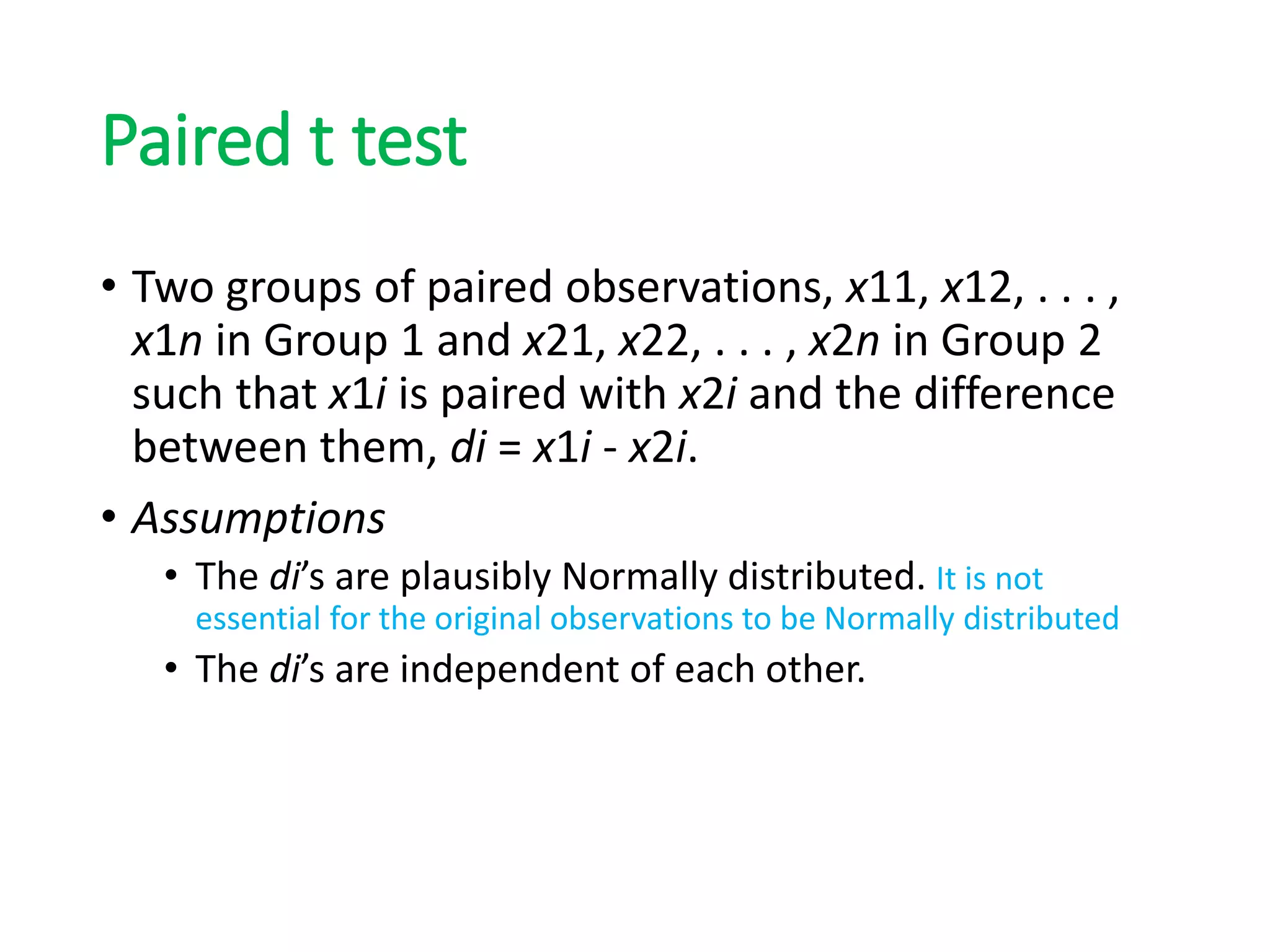
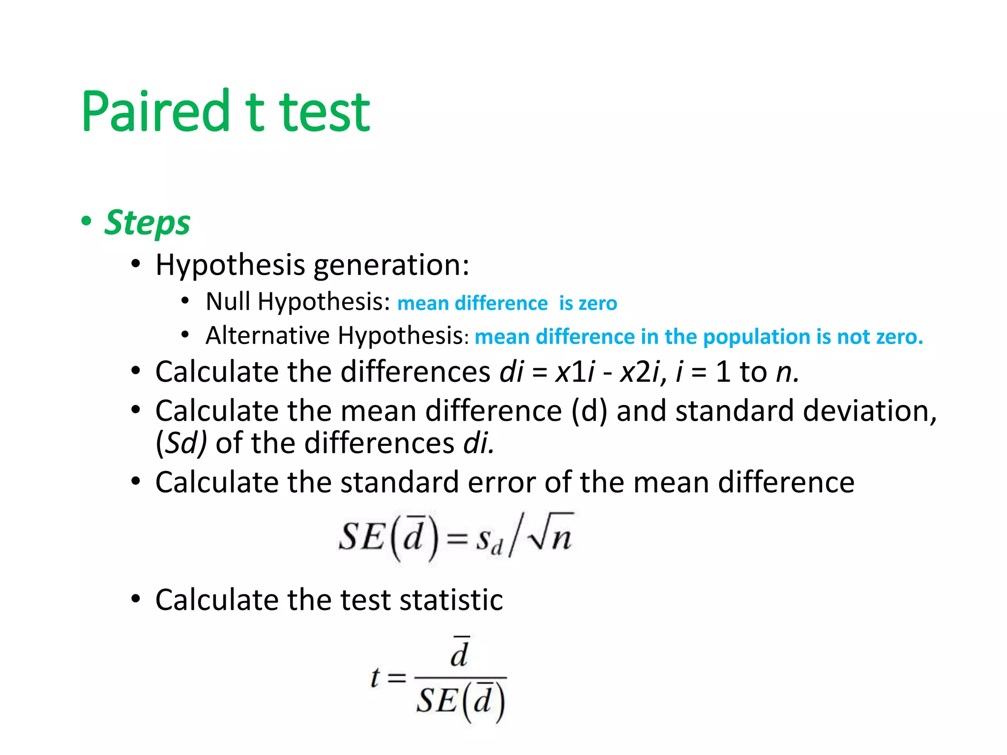
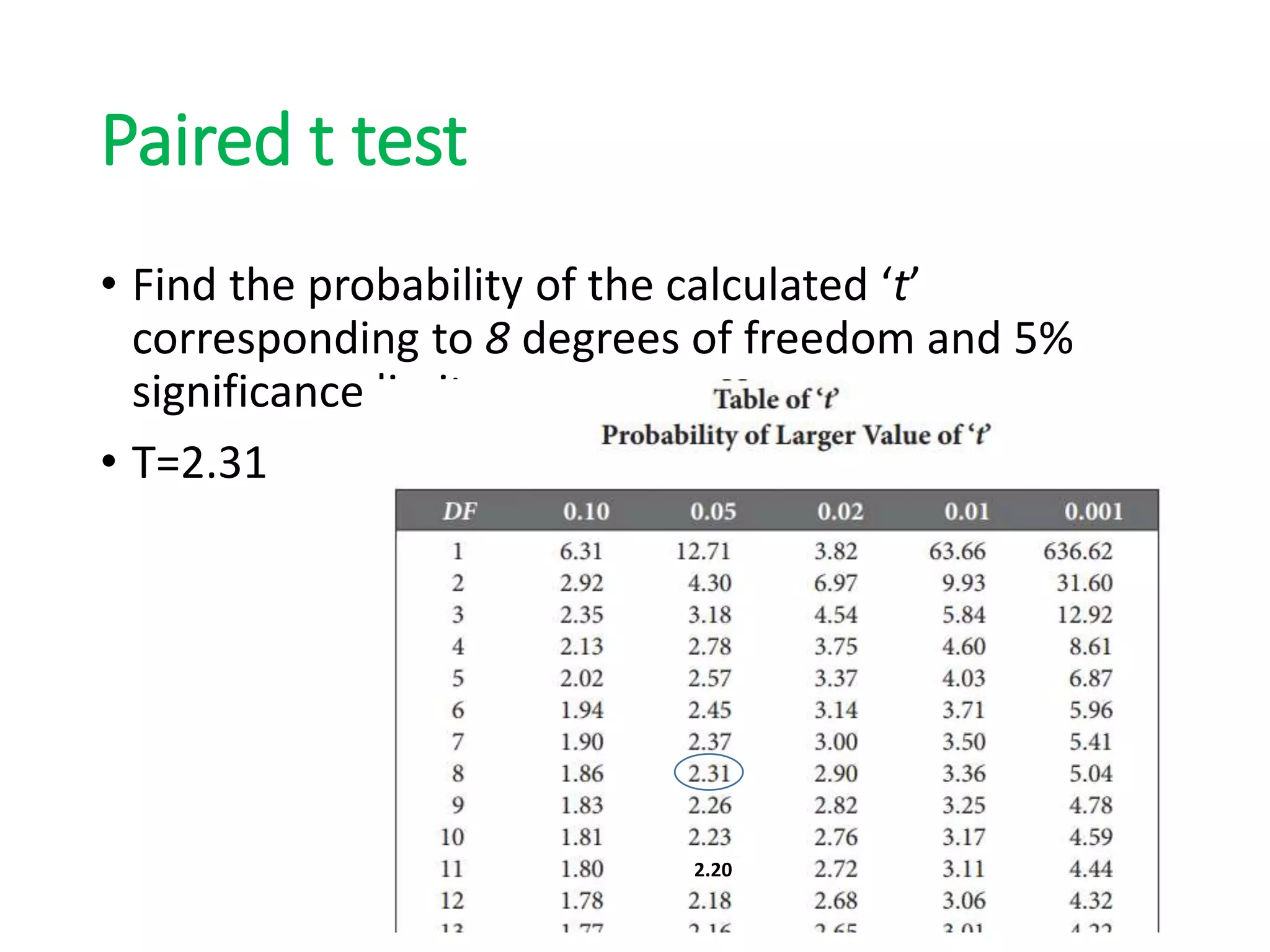
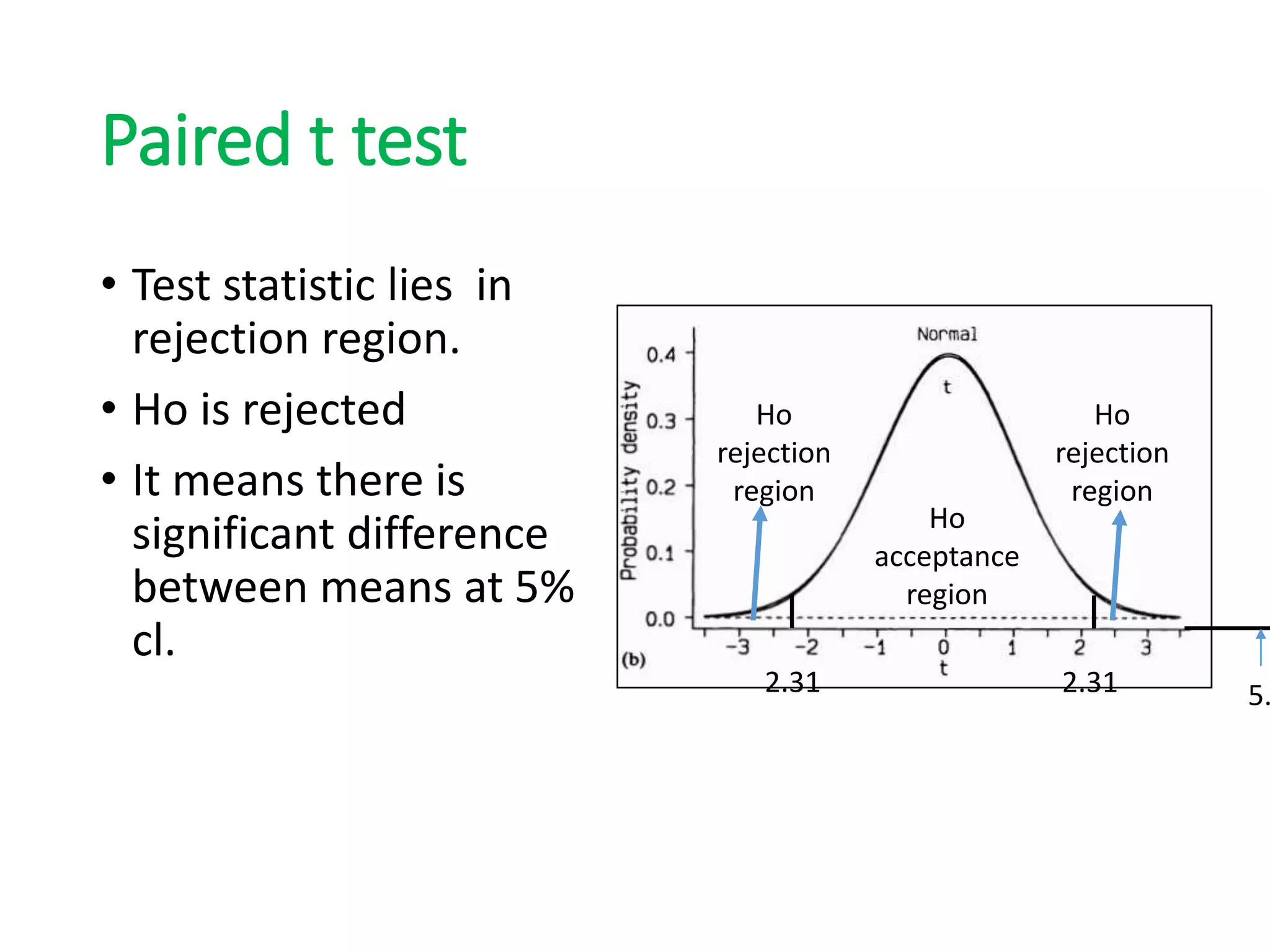
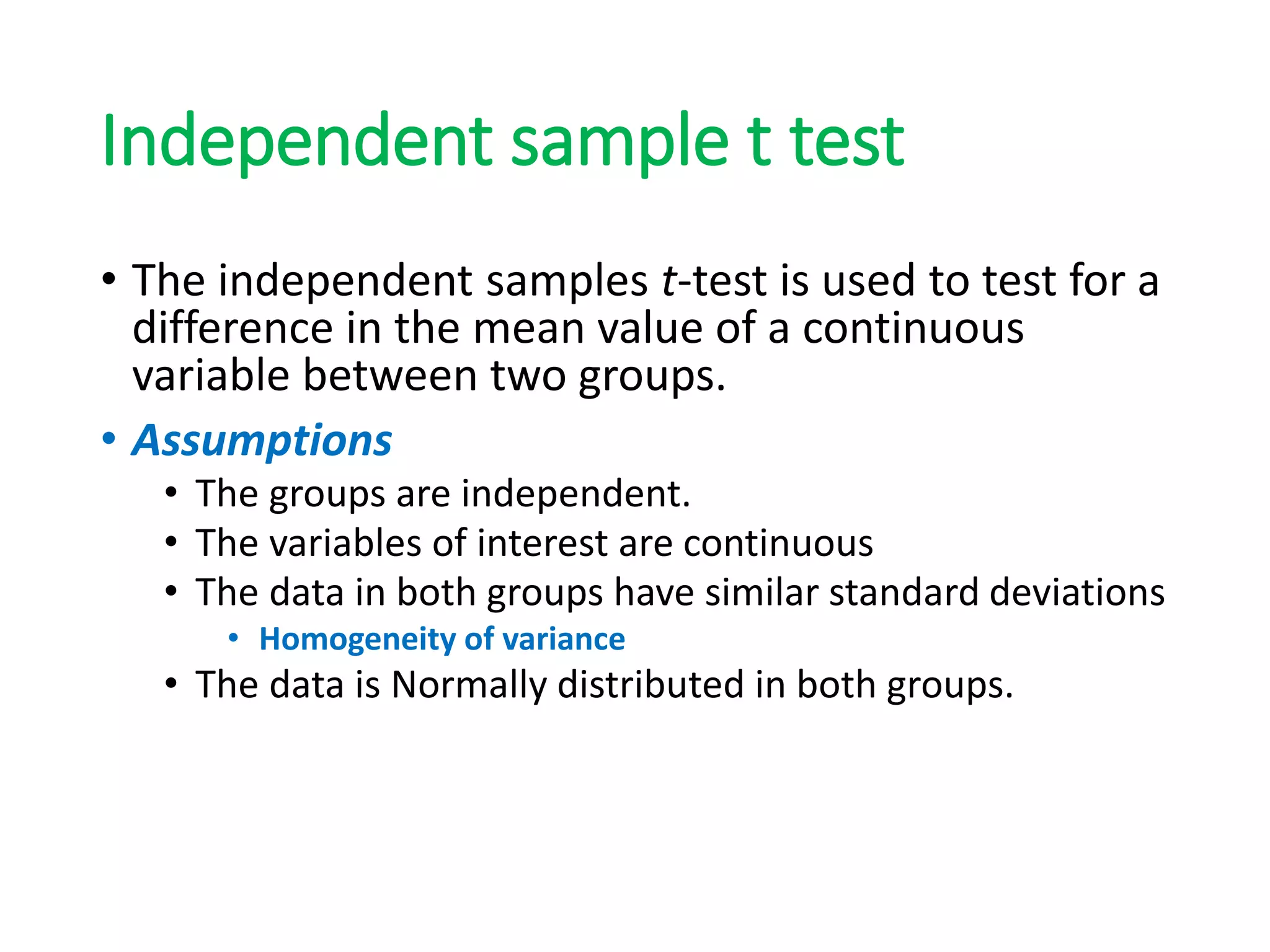


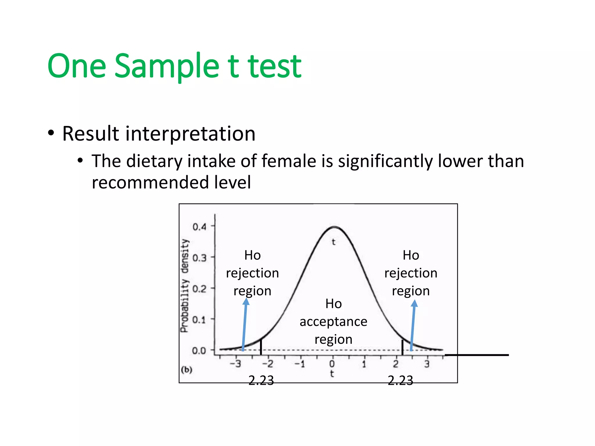


1) The t-test is a statistical test used to determine if there are any statistically significant differences between the means of two groups, and was developed by William Gosset under the pseudonym "Student". 2) The t-distribution is used for calculating t-tests when sample sizes are small and/or variances are unknown. It has a mean of zero and variance greater than one. 3) Paired t-tests are used to compare the means of two related groups when samples are paired, while unpaired t-tests are used to compare unrelated groups or independent samples.