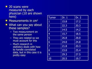
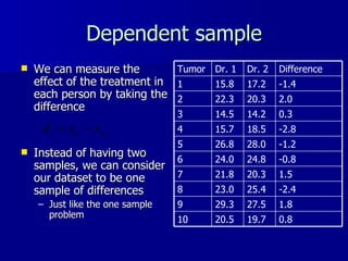
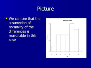
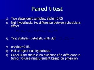
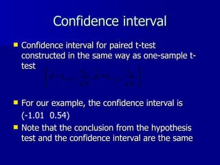
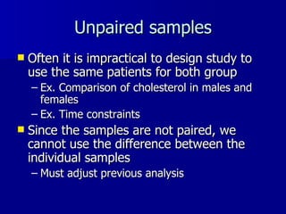
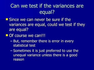
The document discusses comparing measurements from two physicians who measured tumor volumes. A paired t-test was used to test if the measurements significantly differed. The t-test showed no significant difference between physicians. Additionally, two sample t-tests were used to compare tumor volumes between different cancer types, finding significant differences between brain and breast cancers and brain and liver cancers.

1. Comparison of two samples Summer program Brian Healy

2. Previous classes Hypothesis testing Null and Alternative hypotheses Test statistic p-value Conclusion Confidence intervals Comparison of CI to hypothesis test Power and sample size

3. What are we doing today? Two-sample t-test Paired t-test Independent samples Equal variance Unequal variance Sample size for two samples

4. Big picture Up to this point, we have only concerned ourselves with one sample. Often we want to compare one group to another. What happens when we are comparing two samples? Variability in both samples, and potentially two samples are related Much of the theory is the same

5. Example One of the first studies I analyzed was a tumor size study. Having an accurate measure of tumor size is extremely important because it allows a physician to accurately determine if a tumor is growing, shrinking or remaining constant. The problem is that often the measurements of the tumor size vary from physician to physician. In the past, tumor size was measured using the linear distance across the tumor, but this was found to be very variable because of the irregular shape of some tumors. A new method called the RECIST criteria, which traces the outside of the tumor, measures the volume of the tumor. The volumetric method was believed to give more consistent measures of the volume of the tumor.

6. Available data For a portion of the study, a pair of doctors were shown the same set of tumor pictures. The volume of the tumor was measured by two separate physicians under similar conditions. Question of interest: Did the measurements from the two physicians significantly differ? If not, then there would be no evidence that the volume measurements change based on physician.

7. 20 scans were measured by each physician (10 are shown here) Measurements in cm 3 What can you say about these samples? Two measurement on the same person They are related so we must account for this Much research in statistics deals with how to handle correlated data, but in this case it is pretty easy 19.7 20.5 10 27.5 29.3 9 25.4 23.0 8 20.3 21.8 7 24.8 24.0 6 28.0 26.8 5 18.5 15.7 4 14.2 14.5 3 20.3 22.3 2 17.2 15.8 1 Dr. 2 Dr. 1 Tumor

8. Dependent sample We can measure the effect of the treatment in each person by taking the difference Instead of having two samples, we can consider our dataset to be one sample of differences Just like the one sample problem 19.7 27.5 25.4 20.3 24.8 28.0 18.5 14.2 20.3 17.2 Dr. 2 0.8 1.8 -2.4 1.5 -0.8 -1.2 -2.8 0.3 2.0 -1.4 Difference 20.5 10 29.3 9 23.0 8 21.8 7 24.0 6 26.8 5 15.7 4 14.5 3 22.3 2 15.8 1 Dr. 1 Tumor

9. Differences Volume from Dr. 1 Population mean: Sample mean: Volume from Dr. 2 Population mean: Sample mean: Difference Population mean: Sample mean:

10. Distribution of differences Assuming d i ’s are normally distributed, can use t-distribution with n-1 dof where n is the number of differences Standard deviation of differences Test statistic acts just like one sample

11. Picture We can see that the assumption of normality of the differences is reasonable in this case

12. Paired t-test Two dependent samples; alpha=0.05 Null hypothesis: No difference between physicians effect Test statistic: t-statistic with dof p-value=0.53 Fail to reject null hypothesis Conclusion: there is no evidence of a difference in tumor volume measurement based on physician

13. Confidence interval Confidence interval for paired t-test constructed in the same way as one-sample t-test For our example, the confidence interval is (-1.01 0.54) Note that the conclusion from the hypothesis test and the confidence interval are the same

14. Paired t-test in R data<-read.table(G:\\BIO232\\Summer\\pairedscans.dat”, header=F) dr1<-data[,1]; dr2<-data[,2] t.test(dr1, dr2, paired=T) The output provides the p-value and the confidence interval Paired t-test data: data[, 1] and data[, 2] t = -0.6456, df = 19, p-value = 0.5262 alternative hypothesis: true difference in means is not equal to 0 95 percent confidence interval: -1.0180279 0.5380279 sample estimates: mean of the differences -0.24

15. Practice

16. Extensions Some additional examples of paired samples are: Differences between left and right eye Differences between dominant and recessive hand Matched samples When you have more than two samples, techniques account for the correlation between the samples Multivariate / longitudinal data

17. Unpaired samples Often it is impractical to design study to use the same patients for both group Ex. Comparison of cholesterol in males and females Ex. Time constraints Since the samples are not paired, we cannot use the difference between the individual samples Must adjust previous analysis

18. Example Another aspect of the tumor volume study was trying to compare the tumor volume among patients with different forms of cancer. The average tumor size is important to know the effect of treatment can be determined. In this study, patients with brain, breast and liver tumors, but initially we will only compare the brain and breast cancers. All of the tumors were measured using the RECIST method

19. Null hypothesis The null hypothesis is that there is no difference between the volume of the tumor in the two forms of cancer H 0 :  brain  =  breast  , or  brain –  breast =0 More generally, we can test if the difference between two groups is a specific value,  1 -  2 =  This occurs when comparing two treatment groups and we are interested if the two groups are different by a specific amount

20. Each patient contributes one observation Can estimate from the sample Mean and standard deviation in brain cancer group with Mean and standard deviation in breast cancer group with Are the two groups the same? H 0 :  1 =  2 , or  1 -  2 =0 To determine this, we are going to look at We also need to know

21. Difference in the sample means We are going to use the difference of the means as our test statistic, but we need to estimate the variance of this difference to determine if the difference is significant Basic form of test statistic: Standard deviations known unknown The estimate of the standard deviation changes when The samples have equal variance OR The samples have unequal variance

22. Equal variance Sometimes we will be willing to assume that the variance in the two groups is equal: If we know this variance, we can use the z-statistic Often we have to estimate   with the sample variance from each of the samples, Since we have two estimates of one quantity we pool the two estimates

23. Equal variance continued The estimate of  is given by: The t-statistic based on the pooled variance is very similar to the z-statistic as always: The t-statistic has a t-distribution with degrees of freedom

24. For the tumor volume study, there were 20 brain cancer subjects and 28 breast cancer subjects The summary statistics and histogram for the data are given here What can you say about the distributions? Does the equal variance assumption seem valid in this case? 6.0 3.49 s 2 17.5 cm 3 16.2 cm 3 xbar 28 20 n Breast Brain

25. Hypothesis test Two independent samples with equal variance; alpha = 0.05 H 0 : mean brain tumor size = mean breast tumor size p-value: 0.046 Reject null hypothesis Conclusion: There is a significant difference in the size of brain and breast cancer tumors

26. R code If we only had the test statistics above, we can calculate the test statistic and then compare it to the t-distribution using pt(-2.054 ,df=46) to determine the area in the lower tail How do we convert this into the appropriate p-value? With the full data, we can use data<-read.table(“cancer.dat”,header=T) gr<-data[,1]; size<-data[,2] t.test(size[(gr==0)], size[(gr==1)], var.equal=T)

27. R output Two Sample t-test data: size[(gr == 0)] and size[(gr == 1)] t = -2.054, df = 46, p-value = 0.04568 alternative hypothesis: true difference in means is not equal to 0 95 percent confidence interval: -2.65174438 -0.02682705 sample estimates: mean of x mean of y 16.15000 17.48929

28. Unequal variance Often, we are unwilling to assume that the variances are equal We now write the test statistic as: The distribution of this statistic is difficult to derive and we approximate the distribution using a t-distribution with  degrees of freedom

29. This is called the Satterthwaite or Welch approximation When you complete a two-sample t-test in R and the variances are not assumed equal, this approximation is used

30. Example For the comparison of the brain cancers to the liver cancers, the variances are much more different. Let’s use the unequal variance two sample t-test in this case 14.4 3.49 s 2 19.35 cm 3 16.2 cm 3 xbar 20 n Liver Brain

31. Example Two independent samples with equal variance; alpha = 0.05 H 0 : mean brain tumor size = mean liver tumor size p-value: 0.0044 Reject null hypothesis Conclusion: There is a significant difference in the size of the brain and liver tumor size

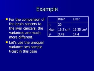
32. R output > t.test(size[(gr==0)],size[(gr==2)]) Welch Two Sample t-test data: size[(gr == 0)] and size[(gr == 2)] t = -3.1666, df = 22.48, p-value = 0.00439 alternative hypothesis: true difference in means is not equal to 0 95 percent confidence interval: -5.288291 -1.105827 sample estimates: mean of x mean of y 16.15000 19.34706

33. Practice Get the dataset from the course folder We want to compare the

34. Can we test if the variances are equal? Since we can never be sure if the variances are equal, could we test if they are equal? Of course we can!!! But, remember there is error in every statistical test Sometimes it is just preferred to use the unequal variance unless there is a good reason

35. Equality of variance H 0 :          To test this hypothesis, we use the sample variances: If one of the variances is much larger than the other, this is evidence against the null As we discussed a couple classes ago:

36. Test of equality One way to test if the two variances are equal is to check if the ratio is equal to 1 Under the null, the ratio simplifies to The ratio of 2 chi-square random variables has an F-distribution The F-distribution is defined by the numerator and denominator degrees of freedom Here we have an F-distribution with n 1 -1 and n 2 -1 degrees of freedom This works better with

37. F-distribution Here is the F-distribution with 5 and 500 degrees of freedom Note the skew of the distribution

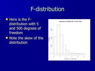
38. Example > var.test(size[(gr==1)],size[(gr==0)]) F test to compare two variances data: size[(gr == 1)] and size[(gr == 0)] F = 1.719, num df = 27, denom df = 19, p-value = 0.2247 alternative hypothesis: true ratio of variances is not equal to 1 95 percent confidence interval: 0.710335 3.904512 sample estimates: ratio of variances 1.719033 > var.test(size[(gr==2)],size[(gr==0)]) F test to compare two variances data: size[(gr == 2)] and size[(gr == 0)] F = 4.1182, num df = 16, denom df = 19, p-value = 0.004156 alternative hypothesis: true ratio of variances is not equal to 1 95 percent confidence interval: 1.589643 11.111060 sample estimates: ratio of variances 4.118214

39. Power and sample size As with the one sample case, we can find power and sample size for a two sample problem For two dependent samples, the power and sample size can be calculated exactly as in the one sample case because the paired t-test is a one sample problem For two independent samples, the power and sample size is slightly different

40. One sample case (review) To find the sample size in the one sample case we needed The hypothesized difference in the means The alpha level The power The variance in the sample One-sided or two sided test

41. Two sample case We still need to have the following pieces of information