Downloaded 129 times

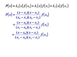
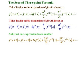
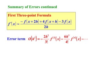
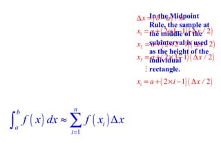
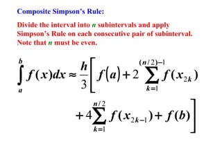
![Using the 1st Three-point formula:
1
{ − 3 f ( x0 ) + 4 f ( x0 + h) − f ( x0 + 2h) }
f ′( x0 ) ≈
2h
1
[ − 3 f ( 2) + 4 f ( 2.1) − f ( 2.2)]
f ′( 2 ) ≈
2 × 0.1
1
[ − 3 × 14.778112 + 4 × 17.148957
=
0.2
− 19.855030 ]
= 22.032310](https://image.slidesharecdn.com/numericaldifferentiationintegration-131111130417-phpapp02/85/Numerical-differentiation-integration-25-320.jpg)
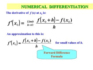
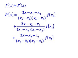
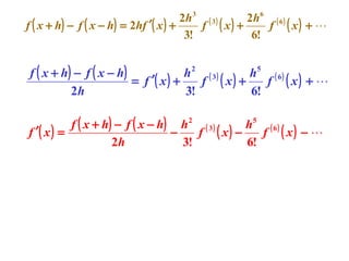
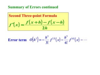
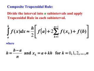
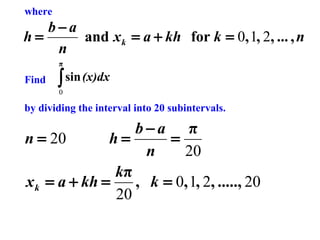
![Using the 2nd Three-point formula:
1
{ f ( x0 + h) − f ( x0 − h) }
f ′( x0 ) ≈
2h
1
[ f ( 2.1) − f (1.9)]
f ′( 2 ) ≈
2 × 0.1
1
[ 17.148957 − 12.703199
=
0.2
= 22.228790
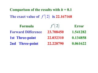
The exact value of
f ′( 2 ) is : 22.167168
]](https://image.slidesharecdn.com/numericaldifferentiationintegration-131111130417-phpapp02/85/Numerical-differentiation-integration-26-320.jpg)
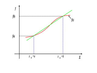
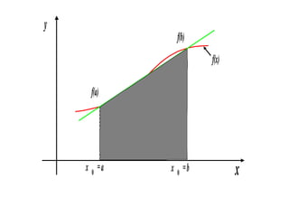
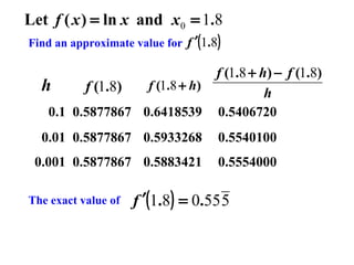
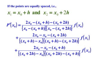
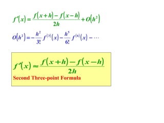
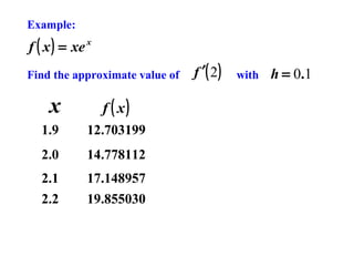
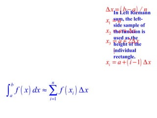
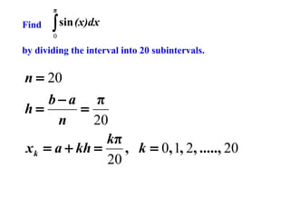
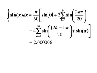
![Area of the trapezoid
The length of the two parallel sides of the trapezoid
are: f(a) and f(b)
The height is b-a
b
∫
a
b−a
[ f ( a ) + f ( b )]
f ( x )dx ≈
2
h
= [ f ( a ) + f ( b )]
2](https://image.slidesharecdn.com/numericaldifferentiationintegration-131111130417-phpapp02/85/Numerical-differentiation-integration-33-320.jpg)
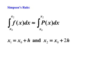
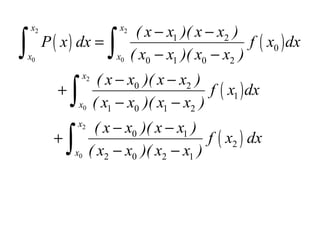
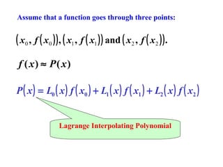
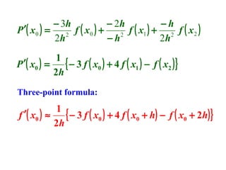
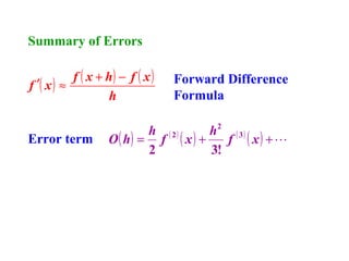
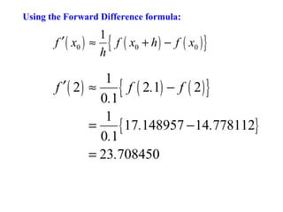
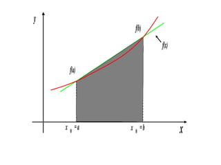
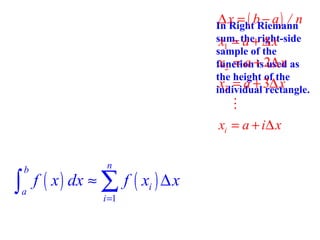
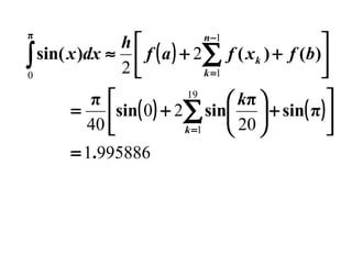
![∫
x2
x0
x2
f ( x )dx ≈ ∫ P ( x )dx
x0
h
= [ f ( x0 ) + 4 f ( x1 ) + f ( x 2 )]
3](https://image.slidesharecdn.com/numericaldifferentiationintegration-131111130417-phpapp02/85/Numerical-differentiation-integration-36-320.jpg)
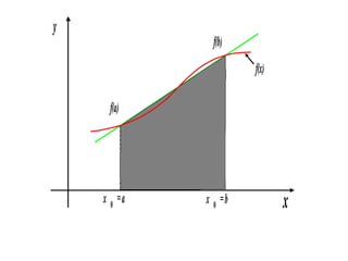
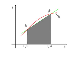
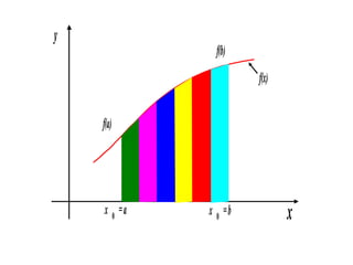

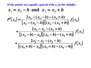
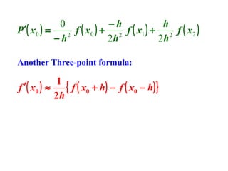
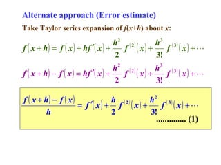
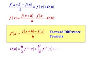
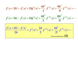
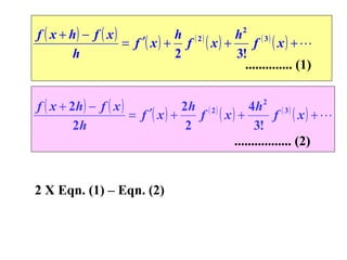
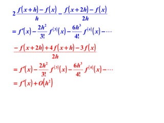
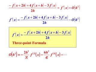
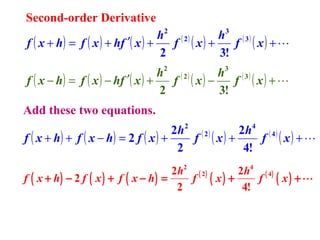
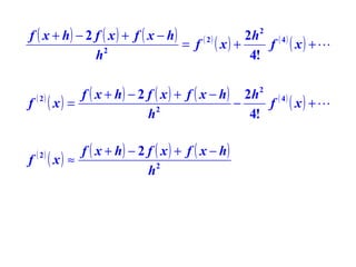
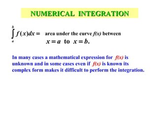
There are several numerical methods described for approximating derivatives and integrals: 1) Forward difference formula approximates the derivative as the slope of the secant line through two nearby points. 2) Three-point formulas approximate the derivative using the slopes of secant lines through three evenly spaced points, reducing the error term to O(h^2). 3) Trapezoidal rule approximates the integral of a function as the area of trapezoids formed between the function graph and the x-axis at evenly spaced points, with error term O(h^2).