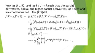
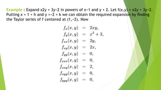
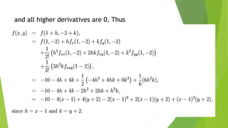
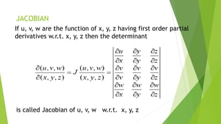
Prepared by :
Vaibhav Tandel (16033010xxxx)
From : Electrical department
Subject : Calculus
Mahatma Gandhi Institute Of Technical
Education And Research Center
Calculus
Applications Of Partial Differentiation
Index
 Taylor’s Theorem for the function of two
variable
 Taylor’s series
 Jacobians
 Errors and Approximation
 Maxima and Minima
 Lagrange’s Method of Undetermined
Multipliers
Taylor's Theorem for Two Variable
Functions
 Rather than go through the arduous development of Taylor's
theorem for functions of two variables, I'll say a few words and
then present the theorem. In the one variable case, the nth term in
the approximation is composed of the nth derivative of the
function.
 For functions of two variables, there are n+1 different derivatives
of nth order. For example, fxxxx, fxxxy, fxxyy, fxyyy, fyyyy are the five
fourth order derivatives.
 There are actually more, but due to the equality of
mixed partial derivatives, many of these are the same.
Thus, our formula for Taylor's theorem must incorporate
more than one derivative at each order.
 The formula for a third order approximation to f(x,y)
near (x0,y0) is
 The factors of 2 and 3 appearing the second and third
order mixed partial terms are due to the fact that there
are two equal mixed partials derivatives of second order
and a pair of three equal third order mixed partials.
 Let U ⊆R, and let f : U →R such that the
derivative, and all the higher derivatives, of f
exist on U. For h∈U,
Taylor series
 This is the Taylor series of f centred at h. If the series is
truncated after n+1 terms we get the Taylor polynomial or
Taylor approximation of f, of degree n, centred at h. If we
replace x with x+h throughout in the Taylor series of f, we
get the following alternative way of expressing the Taylor
series of f centred at h:
 The following are the Taylor series of some standard functions.
The first three are centred at 0, and are valid for all x ∈ R; the
other two are centred at 1, and are valid for x∈R with |x|< 1.
Now let U ⊆ R2, and let f : U → R such that the partial
derivatives, and all the higher partial derivatives, of f exist and
are continuous on U. For (X,Y)∈U,
 and f(r,s) denotes the (r + s)th
partial derivative of f found by differentiating r times with
respect to x and s times with respect to y. This is the Taylor
series of f centred at (X,Y). If the series is truncated after n
+ 1 terms we get the Taylor polynomial or Taylor
approximation of f, of degree n, centred at h.
Example : Expand x2y + 3y−2 in powers of x−1 and y + 2. Let f(x,y) = x2y + 3y−2.
Putting x = 1 + h and y =−2 + k we can obtain the required expansion by finding
the Taylor series of f centered at (1,−2). Now
and all higher derivatives are 0. Thus
If u, v, w are the function of x, y, z having first order partial
derivatives w.r.t. x, y, z then the determinant
JACOBIAN
is called Jacobian of u, v, w w.r.t. x, y, z
Example: Show that when changing to polar coordinates we
have
Solution
So, what we are doing here is justifying the formula that we used
back when we were integrating with respect to polar
coordinates. All that we need to do is use the formula above for
dA.
The transformation here is the standard conversion formulas,
The Jacobian for this transformation is,
Error And Approximation
 Z = f(x , y) be a continuous function of x and y where fᵪ
& fᵧ be the errors occurring in the measurement of the
value of x & y. Then the corresponding error ¶Z occurs
in the estimation of the value of Z.
i.e. Z+¶Z = f(x+¶x , y+¶y)
Therefore, ¶Z = f(x+¶x , y+¶y) – f(x , y).
 Expanding by using Taylor’s Series and neglecting the
higher order terms of ¶x & ¶y, we get,
¶Z = ¶x.¶f/¶x + ¶y.¶f/¶y
 ¶x is known as Absolute Error in x.
 ¶x/x is known as Relative Error in x
 ¶x/x*100 is known as Percentage Error in x.
Example: In measurement of radius of base and height of a
rigid circular cone are incorrect by -1% and 2%. Calculate
Error in the Volume.
Solution,
Let r be the radius and h be the height of the circular cone and
V be the volume of the cone.
V = π/3*r^2*h
Thus,
¶V = ¶r.¶V/¶r + ¶h.¶V/¶h
Now,
¶r/r*100 = -1 ¶h/h*100 = 2
Again,
¶V = π/3(2rh)(r/100) + π/3(r*r)2h/100
= 0
So,
The Error in the measurement in the Volume is Zero.
MAXIMUM & MINIMUM VALUES
 A function f has an absolute maximum
(or global maximum) at c if f(c) ≥ f(x) for
all x in D, where D is the domain of f.
 The number f(c) is called the maximum value of f
on D.
MAXIMUM & MINIMUM VALUES
 Similarly, f has an absolute minimum at c
if f(c) ≤ f(x) for all x in D and the number f(c)
is called the minimum value of f on D.
 The maximum and minimum values of f
are called the extreme values of f.
LOCAL MAXIMUM VALUE
 If we consider only values of x near b—for instance, if we
restrict our attention to the interval (a, c)—then f(b) is the
largest of those values of f(x).
It is called a local
maximum value of f.
LOCAL MINIMUM VALUE
 Likewise, f(c) is called a local minimum value of f because f(c) ≤
f(x) for x near c—for instance, in the interval (b, d).
The function f also has
a local minimum at e.
MAXIMUM & MINIMUM VALUES
 In general, we have the following definition.
 A function f has a local maximum (or relative maximum) at c if f(c) ≥ f(x)
when x is near c.
 This means that f(c) ≥ f(x) for all x in some
open interval containing c.
 Similarly, f has a local minimum at c if f(c) ≤ f(x)
when x is near c.
Lagrange multipliers
 Let U ⊆ R2 and let f,g : U → R. We now consider the
problem of finding the maximum and minimum values
of f subject to the constraint g(x,y) = 0.
Method 1
 Suppose we can rewrite g(x,y) = 0 in the form y = h(x),
for some function h. Then we can just find the
maximum and minimum values of F(x) = f(x,h(x)) using
the method for calculus of functions of one variable.
Example: Find the maximum and minimum values of
f(x,y) = x3 + 3xy2 + 2xy,
subject to the constraint x + y = 4. Here g(x,y) = x + y −4, and g(x,y) = 0
gives y = 4−x. (So h(x) = 4−x.) Thus
Differentiating F with respect to x we get F0(x) = 12x2−52x+56,
and so
For x = 2, y = 2 and F(2) = 40, and for x = 7/3, y = 5/3 and F(7/3) = 39(25/27).
Thus the maximum and minimum values of f(x,y) = x3 + 3xy2 + 2xy, subject
to the constraint x + y = 4, are 40 and 3925 27, respectively.
Method 2
 The local maximum and minimum of f(x,y) subject to
the constraint g(x,y) = 0 correspond to the stationary
points of
L(x,y,λ) = f(x,y)−λg(x,y).
 The variable λ is call a Lagrange multiplier.
Example: Consider the problem from Example 11. Here
f(x,y) = x3 + 3xy2 + 2xy and g(x,y) = x + y−4. So we
let L(x,y,λ) = x3 + 3xy2 + 2xy−λ(x + y−4).
Now,
From equations (1) and (2)
we get, 3x2 + 3y2 + 2y = 6xy + 2x.
We can now use equation (14) to eliminate y form the previous
equation. After simplification this gives
12x2 −52x + 56 = 0
(1)
(3)
(2)
THANK YOU

Applications of partial differentiation

  • 1.
    Prepared by : VaibhavTandel (16033010xxxx) From : Electrical department Subject : Calculus Mahatma Gandhi Institute Of Technical Education And Research Center
  • 2.
  • 3.
    Index  Taylor’s Theoremfor the function of two variable  Taylor’s series  Jacobians  Errors and Approximation  Maxima and Minima  Lagrange’s Method of Undetermined Multipliers
  • 4.
    Taylor's Theorem forTwo Variable Functions  Rather than go through the arduous development of Taylor's theorem for functions of two variables, I'll say a few words and then present the theorem. In the one variable case, the nth term in the approximation is composed of the nth derivative of the function.  For functions of two variables, there are n+1 different derivatives of nth order. For example, fxxxx, fxxxy, fxxyy, fxyyy, fyyyy are the five fourth order derivatives.
  • 5.
     There areactually more, but due to the equality of mixed partial derivatives, many of these are the same. Thus, our formula for Taylor's theorem must incorporate more than one derivative at each order.  The formula for a third order approximation to f(x,y) near (x0,y0) is  The factors of 2 and 3 appearing the second and third order mixed partial terms are due to the fact that there are two equal mixed partials derivatives of second order and a pair of three equal third order mixed partials.
  • 6.
     Let U⊆R, and let f : U →R such that the derivative, and all the higher derivatives, of f exist on U. For h∈U, Taylor series
  • 7.
     This isthe Taylor series of f centred at h. If the series is truncated after n+1 terms we get the Taylor polynomial or Taylor approximation of f, of degree n, centred at h. If we replace x with x+h throughout in the Taylor series of f, we get the following alternative way of expressing the Taylor series of f centred at h:
  • 8.
     The followingare the Taylor series of some standard functions. The first three are centred at 0, and are valid for all x ∈ R; the other two are centred at 1, and are valid for x∈R with |x|< 1.
  • 9.
    Now let U⊆ R2, and let f : U → R such that the partial derivatives, and all the higher partial derivatives, of f exist and are continuous on U. For (X,Y)∈U,
  • 10.
     and f(r,s)denotes the (r + s)th partial derivative of f found by differentiating r times with respect to x and s times with respect to y. This is the Taylor series of f centred at (X,Y). If the series is truncated after n + 1 terms we get the Taylor polynomial or Taylor approximation of f, of degree n, centred at h.
  • 11.
    Example : Expandx2y + 3y−2 in powers of x−1 and y + 2. Let f(x,y) = x2y + 3y−2. Putting x = 1 + h and y =−2 + k we can obtain the required expansion by finding the Taylor series of f centered at (1,−2). Now
  • 12.
    and all higherderivatives are 0. Thus
  • 13.
    If u, v,w are the function of x, y, z having first order partial derivatives w.r.t. x, y, z then the determinant JACOBIAN is called Jacobian of u, v, w w.r.t. x, y, z
  • 14.
    Example: Show thatwhen changing to polar coordinates we have Solution So, what we are doing here is justifying the formula that we used back when we were integrating with respect to polar coordinates. All that we need to do is use the formula above for dA. The transformation here is the standard conversion formulas,
  • 15.
    The Jacobian forthis transformation is,
  • 16.
    Error And Approximation Z = f(x , y) be a continuous function of x and y where fᵪ & fᵧ be the errors occurring in the measurement of the value of x & y. Then the corresponding error ¶Z occurs in the estimation of the value of Z. i.e. Z+¶Z = f(x+¶x , y+¶y) Therefore, ¶Z = f(x+¶x , y+¶y) – f(x , y).
  • 17.
     Expanding byusing Taylor’s Series and neglecting the higher order terms of ¶x & ¶y, we get, ¶Z = ¶x.¶f/¶x + ¶y.¶f/¶y  ¶x is known as Absolute Error in x.  ¶x/x is known as Relative Error in x  ¶x/x*100 is known as Percentage Error in x.
  • 18.
    Example: In measurementof radius of base and height of a rigid circular cone are incorrect by -1% and 2%. Calculate Error in the Volume. Solution, Let r be the radius and h be the height of the circular cone and V be the volume of the cone. V = π/3*r^2*h
  • 19.
    Thus, ¶V = ¶r.¶V/¶r+ ¶h.¶V/¶h Now, ¶r/r*100 = -1 ¶h/h*100 = 2 Again, ¶V = π/3(2rh)(r/100) + π/3(r*r)2h/100 = 0 So, The Error in the measurement in the Volume is Zero.
  • 20.
    MAXIMUM & MINIMUMVALUES  A function f has an absolute maximum (or global maximum) at c if f(c) ≥ f(x) for all x in D, where D is the domain of f.  The number f(c) is called the maximum value of f on D.
  • 21.
    MAXIMUM & MINIMUMVALUES  Similarly, f has an absolute minimum at c if f(c) ≤ f(x) for all x in D and the number f(c) is called the minimum value of f on D.  The maximum and minimum values of f are called the extreme values of f.
  • 22.
    LOCAL MAXIMUM VALUE If we consider only values of x near b—for instance, if we restrict our attention to the interval (a, c)—then f(b) is the largest of those values of f(x). It is called a local maximum value of f.
  • 23.
    LOCAL MINIMUM VALUE Likewise, f(c) is called a local minimum value of f because f(c) ≤ f(x) for x near c—for instance, in the interval (b, d). The function f also has a local minimum at e.
  • 24.
    MAXIMUM & MINIMUMVALUES  In general, we have the following definition.  A function f has a local maximum (or relative maximum) at c if f(c) ≥ f(x) when x is near c.  This means that f(c) ≥ f(x) for all x in some open interval containing c.  Similarly, f has a local minimum at c if f(c) ≤ f(x) when x is near c.
  • 25.
    Lagrange multipliers  LetU ⊆ R2 and let f,g : U → R. We now consider the problem of finding the maximum and minimum values of f subject to the constraint g(x,y) = 0.
  • 26.
    Method 1  Supposewe can rewrite g(x,y) = 0 in the form y = h(x), for some function h. Then we can just find the maximum and minimum values of F(x) = f(x,h(x)) using the method for calculus of functions of one variable.
  • 27.
    Example: Find themaximum and minimum values of f(x,y) = x3 + 3xy2 + 2xy, subject to the constraint x + y = 4. Here g(x,y) = x + y −4, and g(x,y) = 0 gives y = 4−x. (So h(x) = 4−x.) Thus
  • 28.
    Differentiating F withrespect to x we get F0(x) = 12x2−52x+56, and so For x = 2, y = 2 and F(2) = 40, and for x = 7/3, y = 5/3 and F(7/3) = 39(25/27). Thus the maximum and minimum values of f(x,y) = x3 + 3xy2 + 2xy, subject to the constraint x + y = 4, are 40 and 3925 27, respectively.
  • 29.
    Method 2  Thelocal maximum and minimum of f(x,y) subject to the constraint g(x,y) = 0 correspond to the stationary points of L(x,y,λ) = f(x,y)−λg(x,y).  The variable λ is call a Lagrange multiplier.
  • 30.
    Example: Consider theproblem from Example 11. Here f(x,y) = x3 + 3xy2 + 2xy and g(x,y) = x + y−4. So we let L(x,y,λ) = x3 + 3xy2 + 2xy−λ(x + y−4). Now,
  • 31.
    From equations (1)and (2) we get, 3x2 + 3y2 + 2y = 6xy + 2x. We can now use equation (14) to eliminate y form the previous equation. After simplification this gives 12x2 −52x + 56 = 0 (1) (3) (2)
  • 32.