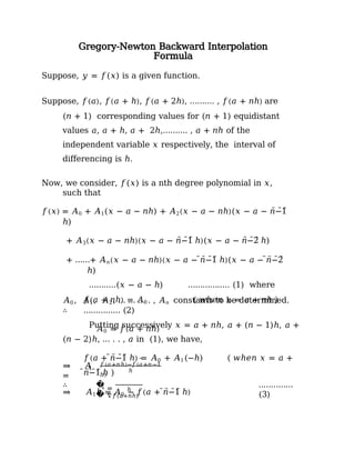
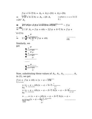
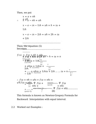
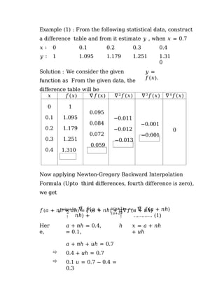
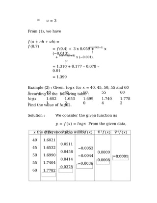
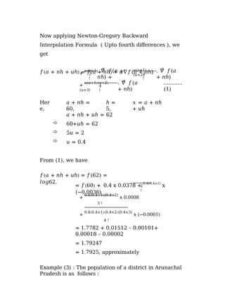
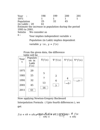
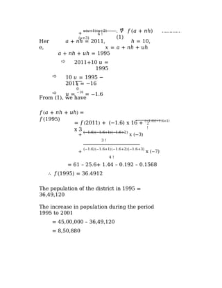
Gregory-Newton
Backward
Interpolation
Formula
Gregory-Newton Backward Interpolation
Formula
Suppose, 𝑦 = 𝑓(𝑥) is a given function.
Suppose, 𝑓(𝑎), 𝑓(𝑎 + ℎ), 𝑓(𝑎 + 2ℎ), ………. , 𝑓(𝑎 + 𝑛ℎ) are
(𝑛 + 1) corresponding values for (𝑛 + 1) equidistant
values 𝑎, 𝑎 + ℎ, 𝑎 + 2ℎ,………. , 𝑎 + 𝑛ℎ of the
independent variable 𝑥 respectively, the interval of
differencing is ℎ.
Now, we consider, 𝑓(𝑥) is a nth degree polynomial in 𝑥,
such that
𝑓(𝑥) = 𝐴0 + 𝐴1(𝑥 − 𝑎 − 𝑛ℎ) + 𝐴2(𝑥 − 𝑎 − 𝑛ℎ)(𝑥 − 𝑎 − 𝑛̅̅̅−̅̅̅1̅
ℎ)
+ 𝐴3(𝑥 − 𝑎 − 𝑛ℎ)(𝑥 − 𝑎 − 𝑛̅̅̅−̅̅̅1̅ ℎ)(𝑥 − 𝑎 − 𝑛̅̅̅−̅̅̅2̅ ℎ)
+ ……+ 𝐴𝑛(𝑥 − 𝑎 − 𝑛ℎ)(𝑥 − 𝑎 − ̅𝑛̅̅−̅̅̅1̅ ℎ)(𝑥 − 𝑎 − ̅𝑛̅̅−̅̅̅2̅
ℎ)
………..(𝑥 − 𝑎 − ℎ) …………….. (1) where
𝐴0 , 𝐴1, 𝐴2, … … … . , 𝐴𝑛 constants to be determined.
Putting successively 𝑥 = 𝑎 + 𝑛ℎ, 𝑎 + (𝑛 − 1)ℎ, 𝑎 +
(𝑛 − 2)ℎ, … . . , 𝑎 in (1), we have,
∴
𝑓(𝑎 + 𝑛ℎ) = 𝐴0 ( 𝑤ℎ𝑒𝑛 𝑥 = 𝑎 + 𝑛ℎ )
…………… (2)
𝐴0 = 𝑓(𝑎 + 𝑛ℎ)
𝑓(𝑎 + ̅𝑛̅̅−̅̅̅1̅ ℎ) = 𝐴0 + 𝐴1(−ℎ) ( 𝑤ℎ𝑒𝑛 𝑥 = 𝑎 +
̅𝑛̅̅−̅̅̅1̅ ℎ )
⇒ 𝐴1ℎ = 𝐴0 − 𝑓(𝑎 + ̅𝑛̅̅−̅̅̅1̅ ℎ)
1
⇒ 𝐴
=
̅̅̅̅̅̅
𝑓(𝑎+𝑛ℎ)−𝑓(𝑎+𝑛−1
ℎ)
ℎ
∴ �
�
1 =
∇𝑓(𝑎+𝑛ℎ)
ℎ
..…………
(3)
𝑓(𝑎 + ̅𝑛̅̅−̅̅̅2̅ ℎ) = 𝐴0 + 𝐴1(−2ℎ) + 𝐴2(−2ℎ)
(−ℎ)
⇒ 𝑓(𝑎 + ̅𝑛̅̅−̅̅̅2̅ ℎ) = 𝐴0 −2ℎ 𝐴1
+2ℎ2
𝐴2
⇒ 2ℎ2
𝐴2 = 𝑓(𝑎 + ̅𝑛̅̅−̅̅̅2̅ ℎ) + 2ℎ. 𝐴1
− 𝐴0
( 𝑤ℎ𝑒𝑛 𝑥 = 𝑎 + ̅𝑛̅̅−̅̅̅2̅
ℎ )
2 ℎ
⇒ 2 ! ℎ2
𝐴 = 𝑓(𝑎 + 𝑛̅̅̅−̅̅̅2̅ ℎ) + 2ℎ.
∇𝑓(𝑎+𝑛ℎ)
− 𝑓(𝑎
+ 𝑛ℎ)
⇒ 2 ! ℎ2
𝐴2 = 𝑓(𝑎 + 𝑛ℎ) − 2𝑓(𝑎 + 𝑛̅̅̅−̅̅̅1̅ ℎ) + 𝑓(𝑎 +
̅𝑛̅̅−̅̅̅2̅ ℎ)
⇒ 2 ! ℎ2
𝐴2 = ∇2
𝑓(𝑎 + 𝑛ℎ)
∴ �
�
2
2
=
∇
𝑓(𝑎+𝑛ℎ)
2 !
ℎ2
..…………
(4)
Similarly, we
get
�
�
3
3
=
∇
𝑓(𝑎+𝑛ℎ)
3 !
ℎ3
�
�
4
4
=
∇
𝑓(𝑎+𝑛ℎ)
4 !
ℎ4
………………
…….
………………
…….
�
�
𝑛
n
=
∇
𝑓(𝑎+𝑛ℎ)
𝑛 !
ℎ𝑛
Now, substituting these values of 𝐴0, 𝐴1, 𝐴2, ……….. , 𝐴𝑛
in (1), we get
𝑓(𝑥) = 𝑓(𝑎 + 𝑛ℎ) + (𝑥 − 𝑎 − 𝑛ℎ)
∇𝑓(𝑎+𝑛ℎ)
ℎ
2
+ (𝑥 − 𝑎 − 𝑛ℎ)(𝑥 − 𝑎 − ̅𝑛̅̅−̅̅̅1̅
ℎ).
∇ 𝑓 (𝑎 +𝑛 ℎ) 2 !
ℎ2 3
+ (𝑥 − 𝑎 − 𝑛ℎ)(𝑥 − 𝑎 − 𝑛̅̅̅−̅̅̅1̅ ℎ)(𝑥 − 𝑎 − 𝑛̅̅̅−̅̅̅2̅
ℎ)
∇ 𝑓(𝑎+𝑛ℎ) 3 ! ℎ3
+ ……+ (𝑥 − 𝑎 − 𝑛ℎ)(𝑥 − 𝑎 − 𝑛̅̅̅−̅̅̅1̅ ℎ)(𝑥 − 𝑎 −
𝑛̅̅̅−̅̅̅2̅ ℎ) 𝑛 !
ℎ𝑛
n
………..(𝑥 − 𝑎 − ℎ)
∇ 𝑓(𝑎+𝑛ℎ)
……………..
(5)
Then, we put
𝑥 = 𝑎 + 𝑛ℎ
+ 𝑢ℎ
∴ 𝑥 − 𝑎 − 𝑛ℎ = 𝑢ℎ
𝑥 − 𝑎 − (𝑛 − 1)ℎ = 𝑢ℎ + ℎ = (𝑢 +
1)ℎ
𝑥 − 𝑎 − (𝑛 − 2)ℎ = 𝑢ℎ + 2ℎ = (𝑢
+ 2)ℎ
…………………………………………………
………..
…………………………………………………
………..
𝑥 − 𝑎 − ℎ = 𝑢ℎ + 𝑛ℎ − ℎ = (𝑢 + 𝑛
− 1)ℎ
Then, the equation (5)
becomes
𝑓(𝑥) = 𝑓(𝑎 + 𝑛ℎ + 𝑢ℎ)
= 𝑓(𝑎 + 𝑛ℎ) + 𝑢ℎ
∇𝑓(𝑎+𝑛ℎ)
ℎ
2
+ 𝑢ℎ(𝑢 + 1)ℎ.
∇
𝑓(𝑎+𝑛ℎ) 2 !
ℎ2 3
+ 𝑢ℎ(𝑢 + 1)ℎ(𝑢 +
2)ℎ.
∇ 𝑓 (𝑎 +𝑛 ℎ ) 3 !
ℎ3 n
+ ……+ 𝑢ℎ(𝑢 + 1)ℎ(𝑢 + 2)ℎ … … (𝑢 + 𝑛
− 1)ℎ
∇ 𝑓 (𝑎 +𝑛 ℎ) 𝑛 !
ℎ𝑛
∴ 𝑓(𝑎 + 𝑛ℎ + 𝑢ℎ) = 𝑓(𝑎 + 𝑛ℎ) +
𝑢∇𝑓(𝑎 + 𝑛ℎ)
+
𝑢(𝑢+1) 2
. ∇ 𝑓(𝑎 +
𝑛ℎ) +
𝑢(𝑢+1)
(𝑢+2)
2 !
3 !
3
. ∇ 𝑓(𝑎
+ 𝑛ℎ)
+ ……. +
𝑢(𝑢+1)(𝑢+2)……
(𝑢+𝑛−1)
𝑛
!
𝑛
. ∇ 𝑓(𝑎 + 𝑛ℎ)……………
(6)
This formula is known as Newton-Gregory Formula for
Backward Interpolation with equal interval.
2.2 Worked out Examples :
Example (1) : From the following statistical data, construct
a difference table and from it estimate 𝑦 , when 𝑥 = 0.7
𝑥 ∶ 0 0.1 0.2 0.3 0.4
𝑦 ∶ 1 1.095 1.179 1.251 1.31
0
Solution : We consider the given
function as From the given data, the
difference table will be
𝑦 =
𝑓(𝑥).
𝑥 𝑓(𝑥) ∇𝑓(𝑥) ∇2
𝑓(𝑥) ∇3
𝑓(𝑥) ∇4
𝑓(𝑥)
0
0.1
0.2
0.3
0.4
1
1.095
1.179
1.251
1.310
0.095
0.084
0.072
0.059
−0.011
−0.012
−0.013
−0.001
−0.001
0
Now applying Newton-Gregory Backward Interpolation
Formula (Upto third differences, fourth difference is zero),
we get
𝑓(𝑎 + 𝑛ℎ + 𝑢ℎ) = 𝑓(𝑎 + 𝑛ℎ) + 𝑢∇𝑓(𝑎 + 𝑛ℎ)
+
𝑢(𝑢+1)
2
!
2
. ∇ 𝑓(𝑎 +
𝑛ℎ) +
𝑢(𝑢+1)
(𝑢+2)
3
!
3
. ∇ 𝑓(𝑎 + 𝑛ℎ)
………… (1)
Her
e,
𝑎 + 𝑛ℎ = 0.4, ℎ
= 0.1,
𝑎 + 𝑛ℎ + 𝑢ℎ = 0.7
 0.4 + 𝑢ℎ = 0.7
 0.1 𝑢 = 0.7 − 0.4 =
0.3
𝑥 = 𝑎 + 𝑛ℎ
+ 𝑢ℎ
 𝑢 = 3
From (1), we have
𝑓(𝑎 + 𝑛ℎ + 𝑢ℎ) =
𝑓(0.7)
2
!
= 𝑓(0.4) + 3 x 0.059 +
3(3+1)
x
(−0.013)
+
3(3+1)(3+2)
x (−0.001)
3 !
= 1.310 + 0.177 – 0.078 –
0.01
= 1.399
Example (2) : Given, 𝑙𝑜𝑔𝑥 for 𝑥 = 40, 45, 50, 55 and 60
according to the following table :
𝑥 ∶
𝑙𝑜𝑔𝑥
∶
40
1.602
1
45
1.653
2
50
1.699
0
55
1.740
4
60
1.778
2
Find the value of 𝑙𝑜𝑔62.
Solution : We consider the given function as
𝑦 = 𝑓(𝑥) = 𝑙𝑜𝑔𝑥 From the given data,
the difference table will be
𝑥 𝑓(𝑥) ∇𝑓(𝑥) ∇2
𝑓(𝑥) ∇3
𝑓(𝑥) ∇4
𝑓(𝑥)
40
45
50
55
60
1.6021
1.6532
1.6990
1.7404
1.7782
0.0511
0.0458
0.0414
0.0378
−0.0053
−0.0044
−0.0036
0.0009
0.0008
−0.0001
Now applying Newton-Gregory Backward
Interpolation Formula ( Upto fourth differences ), we
get
𝑓(𝑎 + 𝑛ℎ + 𝑢ℎ) = 𝑓(𝑎 + 𝑛ℎ) + 𝑢∇𝑓(𝑎 + 𝑛ℎ)
+
𝑢(𝑢+1)
2
!
2
. ∇ 𝑓(𝑎 +
𝑛ℎ) +
𝑢(𝑢+1)
(𝑢+2)
3
!
3
. ∇ 𝑓(𝑎
+ 𝑛ℎ)
+
𝑢(𝑢+1)(𝑢+2)
(𝑢+3)
4
!
4
. ∇ 𝑓(𝑎
+ 𝑛ℎ)
…………
(1)
Her
e,
𝑎 + 𝑛ℎ =
60,
ℎ =
5,
𝑥 = 𝑎 + 𝑛ℎ
+ 𝑢ℎ
𝑎 + 𝑛ℎ + 𝑢ℎ = 62
 60+𝑢ℎ = 62
 5𝑢 = 2
 𝑢 = 0.4
From (1), we have
𝑓(𝑎 + 𝑛ℎ + 𝑢ℎ) = 𝑓(62) =
𝑙𝑜𝑔62.
2
!
= 𝑓(60) + 0.4 x 0.0378 +
0.4(0.4+1)
x
(−0.0036)
+
0.4(0.4+1)(0.4+2)
x 0.0008
3 !
+
0.4(0.4+1)(0.4+2)(0.4+3)
x (−0.0001)
4 !
= 1.7782 + 0.01512 – 0.00101+
0.00018 – 0.00002
= 1.79247
= 1.7925, approximately
Example (3) : The population of a district in Arunachal
Pradesh is as follows :
Year :
1971
Population
(in Lakh) : 20
198
1
199
1
200
1
201
1
25 32 45
61
Estimate the increase in population during the period
1995 to 2001.
Solutio
n :
We consider as
Year implies independent variable 𝑥
Population (in Lakh) implies dependent
variable 𝑦 i.e., 𝑦 = 𝑓(𝑥)
From the given data, the difference
table will be
Year
𝑥
Populati
on in
Lakh
𝑓(𝑥)
∇𝑓(𝑥) ∇2
𝑓(𝑥) ∇3
𝑓(𝑥) ∇4
𝑓(𝑥)
1971
1981
1991
2001
2011
20
25
32
45
61
5
7
13
16
2
6
3
4
−3
−7
Now applying Newton-Gregory Backward
Interpolation Formula ( Upto fourth differences ), we
get
𝑓(𝑎 + 𝑛ℎ + 𝑢ℎ) = 𝑓(𝑎 + 𝑛ℎ) + 𝑢∇𝑓(𝑎 + 𝑛ℎ)
+
𝑢(𝑢+1)
2
!
2
. ∇ 𝑓(𝑎 +
𝑛ℎ) +
𝑢(𝑢+1)
(𝑢+2)
3
!
3
. ∇ 𝑓(𝑎
+ 𝑛ℎ)
+
𝑢(𝑢+1)(𝑢+2)
(𝑢+3)
4
. ∇ 𝑓(𝑎 + 𝑛ℎ) …………
(1)
4 !
𝑎 + 𝑛ℎ = 2011, ℎ = 10,
𝑥 = 𝑎 + 𝑛ℎ + 𝑢ℎ
Her
e,
1
0
𝑎 + 𝑛ℎ + 𝑢ℎ = 1995
 2011+10 𝑢 =
1995
 10 𝑢 = 1995 −
2011 = −16
 𝑢 =
−16
= −1.6
From (1), we have
𝑓(𝑎 + 𝑛ℎ + 𝑢ℎ) =
𝑓(1995)
2
!
= 𝑓(2011) + (−1.6) x 16 + (−1.6)(−1.6+1)
x 3
+
(−1.6)(−1.6+1)(−1.6+2)
x (−3)
3 !
+
(−1.6)(−1.6+1)(−1.6+2)(−1.6+3)
x (−7)
4 !
= 61 – 25.6+ 1.44 – 0.192 – 0.1568
∴ 𝑓(1995) = 36.4912
The population of the district in 1995 =
36,49,120
The increase in population during the period
1995 to 2001
= 45,00,000 – 36,49,120
= 8,50,880

formulanonekjdhdihddhkdddnfdbfdjfkddk.pptx

  • 1.
  • 2.
    Gregory-Newton Backward Interpolation Formula Suppose,𝑦 = 𝑓(𝑥) is a given function. Suppose, 𝑓(𝑎), 𝑓(𝑎 + ℎ), 𝑓(𝑎 + 2ℎ), ………. , 𝑓(𝑎 + 𝑛ℎ) are (𝑛 + 1) corresponding values for (𝑛 + 1) equidistant values 𝑎, 𝑎 + ℎ, 𝑎 + 2ℎ,………. , 𝑎 + 𝑛ℎ of the independent variable 𝑥 respectively, the interval of differencing is ℎ. Now, we consider, 𝑓(𝑥) is a nth degree polynomial in 𝑥, such that 𝑓(𝑥) = 𝐴0 + 𝐴1(𝑥 − 𝑎 − 𝑛ℎ) + 𝐴2(𝑥 − 𝑎 − 𝑛ℎ)(𝑥 − 𝑎 − 𝑛̅̅̅−̅̅̅1̅ ℎ) + 𝐴3(𝑥 − 𝑎 − 𝑛ℎ)(𝑥 − 𝑎 − 𝑛̅̅̅−̅̅̅1̅ ℎ)(𝑥 − 𝑎 − 𝑛̅̅̅−̅̅̅2̅ ℎ) + ……+ 𝐴𝑛(𝑥 − 𝑎 − 𝑛ℎ)(𝑥 − 𝑎 − ̅𝑛̅̅−̅̅̅1̅ ℎ)(𝑥 − 𝑎 − ̅𝑛̅̅−̅̅̅2̅ ℎ) ………..(𝑥 − 𝑎 − ℎ) …………….. (1) where 𝐴0 , 𝐴1, 𝐴2, … … … . , 𝐴𝑛 constants to be determined. Putting successively 𝑥 = 𝑎 + 𝑛ℎ, 𝑎 + (𝑛 − 1)ℎ, 𝑎 + (𝑛 − 2)ℎ, … . . , 𝑎 in (1), we have, ∴ 𝑓(𝑎 + 𝑛ℎ) = 𝐴0 ( 𝑤ℎ𝑒𝑛 𝑥 = 𝑎 + 𝑛ℎ ) …………… (2) 𝐴0 = 𝑓(𝑎 + 𝑛ℎ) 𝑓(𝑎 + ̅𝑛̅̅−̅̅̅1̅ ℎ) = 𝐴0 + 𝐴1(−ℎ) ( 𝑤ℎ𝑒𝑛 𝑥 = 𝑎 + ̅𝑛̅̅−̅̅̅1̅ ℎ ) ⇒ 𝐴1ℎ = 𝐴0 − 𝑓(𝑎 + ̅𝑛̅̅−̅̅̅1̅ ℎ) 1 ⇒ 𝐴 = ̅̅̅̅̅̅ 𝑓(𝑎+𝑛ℎ)−𝑓(𝑎+𝑛−1 ℎ) ℎ ∴ � � 1 = ∇𝑓(𝑎+𝑛ℎ) ℎ ..………… (3)
  • 3.
    𝑓(𝑎 + ̅𝑛̅̅−̅̅̅2̅ℎ) = 𝐴0 + 𝐴1(−2ℎ) + 𝐴2(−2ℎ) (−ℎ) ⇒ 𝑓(𝑎 + ̅𝑛̅̅−̅̅̅2̅ ℎ) = 𝐴0 −2ℎ 𝐴1 +2ℎ2 𝐴2 ⇒ 2ℎ2 𝐴2 = 𝑓(𝑎 + ̅𝑛̅̅−̅̅̅2̅ ℎ) + 2ℎ. 𝐴1 − 𝐴0 ( 𝑤ℎ𝑒𝑛 𝑥 = 𝑎 + ̅𝑛̅̅−̅̅̅2̅ ℎ ) 2 ℎ ⇒ 2 ! ℎ2 𝐴 = 𝑓(𝑎 + 𝑛̅̅̅−̅̅̅2̅ ℎ) + 2ℎ. ∇𝑓(𝑎+𝑛ℎ) − 𝑓(𝑎 + 𝑛ℎ) ⇒ 2 ! ℎ2 𝐴2 = 𝑓(𝑎 + 𝑛ℎ) − 2𝑓(𝑎 + 𝑛̅̅̅−̅̅̅1̅ ℎ) + 𝑓(𝑎 + ̅𝑛̅̅−̅̅̅2̅ ℎ) ⇒ 2 ! ℎ2 𝐴2 = ∇2 𝑓(𝑎 + 𝑛ℎ) ∴ � � 2 2 = ∇ 𝑓(𝑎+𝑛ℎ) 2 ! ℎ2 ..………… (4) Similarly, we get � � 3 3 = ∇ 𝑓(𝑎+𝑛ℎ) 3 ! ℎ3 � � 4 4 = ∇ 𝑓(𝑎+𝑛ℎ) 4 ! ℎ4 ……………… ……. ……………… ……. � � 𝑛 n = ∇ 𝑓(𝑎+𝑛ℎ) 𝑛 ! ℎ𝑛 Now, substituting these values of 𝐴0, 𝐴1, 𝐴2, ……….. , 𝐴𝑛 in (1), we get 𝑓(𝑥) = 𝑓(𝑎 + 𝑛ℎ) + (𝑥 − 𝑎 − 𝑛ℎ) ∇𝑓(𝑎+𝑛ℎ) ℎ 2 + (𝑥 − 𝑎 − 𝑛ℎ)(𝑥 − 𝑎 − ̅𝑛̅̅−̅̅̅1̅ ℎ). ∇ 𝑓 (𝑎 +𝑛 ℎ) 2 ! ℎ2 3 + (𝑥 − 𝑎 − 𝑛ℎ)(𝑥 − 𝑎 − 𝑛̅̅̅−̅̅̅1̅ ℎ)(𝑥 − 𝑎 − 𝑛̅̅̅−̅̅̅2̅ ℎ) ∇ 𝑓(𝑎+𝑛ℎ) 3 ! ℎ3 + ……+ (𝑥 − 𝑎 − 𝑛ℎ)(𝑥 − 𝑎 − 𝑛̅̅̅−̅̅̅1̅ ℎ)(𝑥 − 𝑎 − 𝑛̅̅̅−̅̅̅2̅ ℎ) 𝑛 ! ℎ𝑛 n ………..(𝑥 − 𝑎 − ℎ) ∇ 𝑓(𝑎+𝑛ℎ) …………….. (5)
  • 4.
    Then, we put 𝑥= 𝑎 + 𝑛ℎ + 𝑢ℎ ∴ 𝑥 − 𝑎 − 𝑛ℎ = 𝑢ℎ 𝑥 − 𝑎 − (𝑛 − 1)ℎ = 𝑢ℎ + ℎ = (𝑢 + 1)ℎ 𝑥 − 𝑎 − (𝑛 − 2)ℎ = 𝑢ℎ + 2ℎ = (𝑢 + 2)ℎ ………………………………………………… ……….. ………………………………………………… ……….. 𝑥 − 𝑎 − ℎ = 𝑢ℎ + 𝑛ℎ − ℎ = (𝑢 + 𝑛 − 1)ℎ Then, the equation (5) becomes 𝑓(𝑥) = 𝑓(𝑎 + 𝑛ℎ + 𝑢ℎ) = 𝑓(𝑎 + 𝑛ℎ) + 𝑢ℎ ∇𝑓(𝑎+𝑛ℎ) ℎ 2 + 𝑢ℎ(𝑢 + 1)ℎ. ∇ 𝑓(𝑎+𝑛ℎ) 2 ! ℎ2 3 + 𝑢ℎ(𝑢 + 1)ℎ(𝑢 + 2)ℎ. ∇ 𝑓 (𝑎 +𝑛 ℎ ) 3 ! ℎ3 n + ……+ 𝑢ℎ(𝑢 + 1)ℎ(𝑢 + 2)ℎ … … (𝑢 + 𝑛 − 1)ℎ ∇ 𝑓 (𝑎 +𝑛 ℎ) 𝑛 ! ℎ𝑛 ∴ 𝑓(𝑎 + 𝑛ℎ + 𝑢ℎ) = 𝑓(𝑎 + 𝑛ℎ) + 𝑢∇𝑓(𝑎 + 𝑛ℎ) + 𝑢(𝑢+1) 2 . ∇ 𝑓(𝑎 + 𝑛ℎ) + 𝑢(𝑢+1) (𝑢+2) 2 ! 3 ! 3 . ∇ 𝑓(𝑎 + 𝑛ℎ) + ……. + 𝑢(𝑢+1)(𝑢+2)…… (𝑢+𝑛−1) 𝑛 ! 𝑛 . ∇ 𝑓(𝑎 + 𝑛ℎ)…………… (6) This formula is known as Newton-Gregory Formula for Backward Interpolation with equal interval. 2.2 Worked out Examples :
  • 5.
    Example (1) :From the following statistical data, construct a difference table and from it estimate 𝑦 , when 𝑥 = 0.7 𝑥 ∶ 0 0.1 0.2 0.3 0.4 𝑦 ∶ 1 1.095 1.179 1.251 1.31 0 Solution : We consider the given function as From the given data, the difference table will be 𝑦 = 𝑓(𝑥). 𝑥 𝑓(𝑥) ∇𝑓(𝑥) ∇2 𝑓(𝑥) ∇3 𝑓(𝑥) ∇4 𝑓(𝑥) 0 0.1 0.2 0.3 0.4 1 1.095 1.179 1.251 1.310 0.095 0.084 0.072 0.059 −0.011 −0.012 −0.013 −0.001 −0.001 0 Now applying Newton-Gregory Backward Interpolation Formula (Upto third differences, fourth difference is zero), we get 𝑓(𝑎 + 𝑛ℎ + 𝑢ℎ) = 𝑓(𝑎 + 𝑛ℎ) + 𝑢∇𝑓(𝑎 + 𝑛ℎ) + 𝑢(𝑢+1) 2 ! 2 . ∇ 𝑓(𝑎 + 𝑛ℎ) + 𝑢(𝑢+1) (𝑢+2) 3 ! 3 . ∇ 𝑓(𝑎 + 𝑛ℎ) ………… (1) Her e, 𝑎 + 𝑛ℎ = 0.4, ℎ = 0.1, 𝑎 + 𝑛ℎ + 𝑢ℎ = 0.7  0.4 + 𝑢ℎ = 0.7  0.1 𝑢 = 0.7 − 0.4 = 0.3 𝑥 = 𝑎 + 𝑛ℎ + 𝑢ℎ
  • 6.
     𝑢 =3 From (1), we have 𝑓(𝑎 + 𝑛ℎ + 𝑢ℎ) = 𝑓(0.7) 2 ! = 𝑓(0.4) + 3 x 0.059 + 3(3+1) x (−0.013) + 3(3+1)(3+2) x (−0.001) 3 ! = 1.310 + 0.177 – 0.078 – 0.01 = 1.399 Example (2) : Given, 𝑙𝑜𝑔𝑥 for 𝑥 = 40, 45, 50, 55 and 60 according to the following table : 𝑥 ∶ 𝑙𝑜𝑔𝑥 ∶ 40 1.602 1 45 1.653 2 50 1.699 0 55 1.740 4 60 1.778 2 Find the value of 𝑙𝑜𝑔62. Solution : We consider the given function as 𝑦 = 𝑓(𝑥) = 𝑙𝑜𝑔𝑥 From the given data, the difference table will be 𝑥 𝑓(𝑥) ∇𝑓(𝑥) ∇2 𝑓(𝑥) ∇3 𝑓(𝑥) ∇4 𝑓(𝑥) 40 45 50 55 60 1.6021 1.6532 1.6990 1.7404 1.7782 0.0511 0.0458 0.0414 0.0378 −0.0053 −0.0044 −0.0036 0.0009 0.0008 −0.0001
  • 7.
    Now applying Newton-GregoryBackward Interpolation Formula ( Upto fourth differences ), we get 𝑓(𝑎 + 𝑛ℎ + 𝑢ℎ) = 𝑓(𝑎 + 𝑛ℎ) + 𝑢∇𝑓(𝑎 + 𝑛ℎ) + 𝑢(𝑢+1) 2 ! 2 . ∇ 𝑓(𝑎 + 𝑛ℎ) + 𝑢(𝑢+1) (𝑢+2) 3 ! 3 . ∇ 𝑓(𝑎 + 𝑛ℎ) + 𝑢(𝑢+1)(𝑢+2) (𝑢+3) 4 ! 4 . ∇ 𝑓(𝑎 + 𝑛ℎ) ………… (1) Her e, 𝑎 + 𝑛ℎ = 60, ℎ = 5, 𝑥 = 𝑎 + 𝑛ℎ + 𝑢ℎ 𝑎 + 𝑛ℎ + 𝑢ℎ = 62  60+𝑢ℎ = 62  5𝑢 = 2  𝑢 = 0.4 From (1), we have 𝑓(𝑎 + 𝑛ℎ + 𝑢ℎ) = 𝑓(62) = 𝑙𝑜𝑔62. 2 ! = 𝑓(60) + 0.4 x 0.0378 + 0.4(0.4+1) x (−0.0036) + 0.4(0.4+1)(0.4+2) x 0.0008 3 ! + 0.4(0.4+1)(0.4+2)(0.4+3) x (−0.0001) 4 ! = 1.7782 + 0.01512 – 0.00101+ 0.00018 – 0.00002 = 1.79247 = 1.7925, approximately Example (3) : The population of a district in Arunachal Pradesh is as follows :
  • 8.
    Year : 1971 Population (in Lakh): 20 198 1 199 1 200 1 201 1 25 32 45 61 Estimate the increase in population during the period 1995 to 2001. Solutio n : We consider as Year implies independent variable 𝑥 Population (in Lakh) implies dependent variable 𝑦 i.e., 𝑦 = 𝑓(𝑥) From the given data, the difference table will be Year 𝑥 Populati on in Lakh 𝑓(𝑥) ∇𝑓(𝑥) ∇2 𝑓(𝑥) ∇3 𝑓(𝑥) ∇4 𝑓(𝑥) 1971 1981 1991 2001 2011 20 25 32 45 61 5 7 13 16 2 6 3 4 −3 −7 Now applying Newton-Gregory Backward Interpolation Formula ( Upto fourth differences ), we get 𝑓(𝑎 + 𝑛ℎ + 𝑢ℎ) = 𝑓(𝑎 + 𝑛ℎ) + 𝑢∇𝑓(𝑎 + 𝑛ℎ) + 𝑢(𝑢+1) 2 ! 2 . ∇ 𝑓(𝑎 + 𝑛ℎ) + 𝑢(𝑢+1) (𝑢+2) 3 ! 3 . ∇ 𝑓(𝑎 + 𝑛ℎ)
  • 9.
    + 𝑢(𝑢+1)(𝑢+2) (𝑢+3) 4 . ∇ 𝑓(𝑎+ 𝑛ℎ) ………… (1) 4 ! 𝑎 + 𝑛ℎ = 2011, ℎ = 10, 𝑥 = 𝑎 + 𝑛ℎ + 𝑢ℎ Her e, 1 0 𝑎 + 𝑛ℎ + 𝑢ℎ = 1995  2011+10 𝑢 = 1995  10 𝑢 = 1995 − 2011 = −16  𝑢 = −16 = −1.6 From (1), we have 𝑓(𝑎 + 𝑛ℎ + 𝑢ℎ) = 𝑓(1995) 2 ! = 𝑓(2011) + (−1.6) x 16 + (−1.6)(−1.6+1) x 3 + (−1.6)(−1.6+1)(−1.6+2) x (−3) 3 ! + (−1.6)(−1.6+1)(−1.6+2)(−1.6+3) x (−7) 4 ! = 61 – 25.6+ 1.44 – 0.192 – 0.1568 ∴ 𝑓(1995) = 36.4912 The population of the district in 1995 = 36,49,120 The increase in population during the period 1995 to 2001 = 45,00,000 – 36,49,120 = 8,50,880