This document discusses intervals of validity for solutions to differential equations. It presents two theorems, one for linear first-order equations and one for non-linear equations. The linear theorem guarantees a unique solution over intervals where coefficients are continuous, allowing validity intervals to be found without solving the equation. However, for non-linear equations the solution must be found to determine the validity interval, which can depend on the initial condition. Examples illustrate finding validity intervals, the possibility of multiple solutions if theorem conditions are violated, and how validity intervals can depend on initial conditions for non-linear equations.

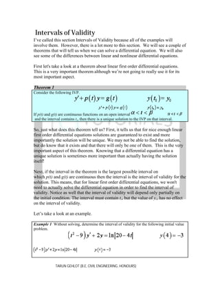
1. Intervals of Validity
I’ve called this section Intervals of Validity because all of the examples will
involve them. However, there is a lot more to this section. We will see a couple of
theorems that will tell us when we can solve a differential equation. We will also
see some of the differences between linear and nonlinear differential equations.
First let's take a look at a theorem about linear first order differential equations.
This is a very important theorem although we’re not going to really use it for its
most important aspect.
Theorem 1
Consider the following IVP.
If p(t) and g(t) are continuous functions on an open interval
and the interval contains to, then there is a unique solution to the IVP on that interval.
So, just what does this theorem tell us? First, it tells us that for nice enough linear
first order differential equations solutions are guaranteed to exist and more
importantly the solution will be unique. We may not be able to find the solution,
but do know that it exists and that there will only be one of them. This is the very
important aspect of this theorem. Knowing that a differential equation has a
unique solution is sometimes more important than actually having the solution
itself!
Next, if the interval in the theorem is the largest possible interval on
which p(t) and g(t) are continuous then the interval is the interval of validity for the
solution. This means, that for linear first order differential equations, we won't
need to actually solve the differential equation in order to find the interval of
validity. Notice as well that the interval of validity will depend only partially on
the initial condition. The interval must contain to, but the value of yo, has no effect
on the interval of validity.
Let’s take a look at an example.
Example 1 Without solving, determine the interval of validity for the following initial value
problem.
TARUN GEHLOT (B.E, CIVIL ENGINEERING, HONOURS)

2. Solution
First, in order to use the theorem to find the interval of validity we must write the differential
equation in the proper form given in the theorem. So we will need to divide out by the
coefficient of the derivative.
Next, we need to identify where the two functions are not continuous. This will allow us to
find all possible intervals of validity for the differential equation. So, p(t) will be
discontinuous at
since these points will give a division by zero.
Likewise, g(t) will also be discontinuous at
as well as t = 5 since at
this point we will have the natural logarithm of zero. Note that in this case we won't have to
worry about natural log of negative numbers because of the absolute values.
Now, with these points in hand we can break up the real number line into four intervals where
both p(t) and g(t) will be continuous. These four intervals are,
The endpoints of each of the intervals are points where at least one of the two functions is
discontinuous. This will guarantee that both functions are continuous everywhere in each
interval.
Finally, let's identify the actual interval of validity for the initial value problem. The actual
interval of validity is the interval that will contain to = 4. So, the interval of validity for the
initial value problem is.
In this last example we need to be careful to not jump to the conclusion that the
other three intervals cannot be intervals of validity. By changing the initial
condition, in particular the value of to, we can make any of the four intervals the
interval of validity.
The first theorem required a linear differential equation. There is a similar theorem
for non-linear first order differential equations. This theorem is not as useful for
finding intervals of validity as the first theorem was so we won’t be doing all that
much with it.
Here is the theorem.
Theorem 2
TARUN GEHLOT (B.E, CIVIL ENGINEERING, HONOURS)

3. Consider the following IVP.
If f(t,y) and
are continuous functions in some rectangle
,
containing the point (to, yo) then there is a unique
solution to the IVP in some interval to
h < t < to + h that is contained in

That’s it. Unlike the first theorem, this one cannot really be used to find an
interval of validity. So, we will know that a unique solution exists if the conditions
of the theorem are met, but we will actually need the solution in order to determine
its interval of validity. Note as well that for non-linear differential equations it
appears that the value of y0 may affect the interval of validity.
Here is an example of the problems that can arise when the conditions of this
theorem aren’t met.
Example 2 Determine all possible solutions to the following IVP.
Solution
First, notice that this differential equation does NOT satisfy the conditions of the theorem.
So, the function is continuous on any interval, but the derivative is not continuous at y = 0
and so will not be continuous at any interval containing y = 0. In order to use the theorem
both must be continuous on an interval that contains yo = 0 and this is problem for us since we
do have yo = 0.
Now, let’s actually work the problem. This differential equation is separable and is fairly
simple to solve.
TARUN GEHLOT (B.E, CIVIL ENGINEERING, HONOURS)

4. Applying the initial condition gives c = 0 and so the solution is.
So, we’ve got two possible solutions here, both of which satisfy the differential equation and
the initial condition. There is also a third solution to the IVP. y(t) = 0 is also a solution to
the differential equation and satisfies the initial condition.
In this last example we had a very simple IVP and it only violated one of the
conditions of the theorem, yet it had three different solutions. All the examples
we’ve worked in the previous sections satisfied the conditions of this theorem and
had a single unique solution to the IVP. This example is a useful reminder of the
fact that, in the field of differential equations, things don’t always behave nicely.
It’s easy to forget this as most of the problems that are worked in a differential
equations class are nice and behave in a nice, predictable manner.
Let’s work one final example that will illustrate one of the differences between
linear and non-linear differential equations.
Example 3 Determine the interval of validity for the initial value problem below and give its
dependence on the value of yo
Solution
Before proceeding in this problem, we should note that the differential equation is non-linear
and meets both conditions of the Theorem 2 and so there will be a unique solution to the IVP
for each possible value of yo.
Also, note that the problem asks for any dependence of the interval of validity on the value
of yo. This immediately illustrates a difference between linear and non-linear differential
equations. Intervals of validity for linear differential equations do not depend on the value
of yo. Intervals of validity for non-linear differential can depend on the value of yo as we
pointed out after the second theorem.
TARUN GEHLOT (B.E, CIVIL ENGINEERING, HONOURS)

5. So, let’s solve the IVP and get some intervals of validity.
First note that if yo = 0 then y(t) = 0 is the solution and this has an interval of validity of
So for the rest of the problem let's assume that
equation is separable so let's solve it and get a general solution.
. Now, the differential
Applying the initial condition gives
The solution is then.
Now that we have a solution to the initial value problem we can start finding intervals of
validity. From the solution we can see that the only problem that we’ll have is division by
zero at
This leads to two possible intervals of validity.
That actual interval of validity will be the interval that contains to = 0. This however, depends
TARUN GEHLOT (B.E, CIVIL ENGINEERING, HONOURS)

6. on the value of yo. If yo < 0 then
contain to = 0. Likewise if yo > 0 then
will contain to = 0.
and so the second interval will
and in this case the first interval
This leads to the following possible intervals of validity, depending on the value of yo.
On a side note, notice that the solution, in its final form, will also work if yo = 0.
So what did this example show us about the difference between linear and nonlinear differential equations?
First, as pointed out in the solution to the example, intervals of validity for nonlinear differential equations can depend on the value of yo, whereas intervals of
validity for linear differential equations don’t.
Second, intervals of validity for linear differential equations can be found from the
differential equation with no knowledge of the solution. This is definitely not the
case with non-linear differential equations. It would be very difficult to see how
any of these intervals in the last example could be found from the differential
equation. Knowledge of the solution was required in order for us to find the
interval of validity.
TARUN GEHLOT (B.E, CIVIL ENGINEERING, HONOURS)