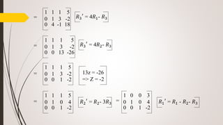
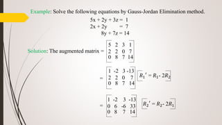
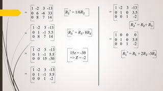
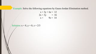
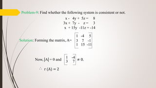
Downloaded 11 times

![Method of False Position
(0,0)
X
Y
[a, f(a)]
[b, f(b)]
f(x) 𝑦−𝑓(𝑎)
𝑥−𝑎
=
𝑓 𝑏 − 𝑓(𝑎)
𝑏−𝑎
Let, y = 0,
−𝑓(𝑎)
𝑥−𝑎
=
𝑓 𝑏 − 𝑓(𝑎)
𝑏−𝑎
x-a = -
(𝑏−𝑎)𝑓(𝑎)
𝑓 𝑏 −𝑓(𝑎)
x = a -
(𝑏−𝑎)𝑓(𝑎)
𝑓 𝑏 −𝑓(𝑎)
Derive the root of a curve f(x) by False Position method.](https://image.slidesharecdn.com/ce205-200326191144/85/Numerical-Methods-and-Analysis-11-320.jpg)

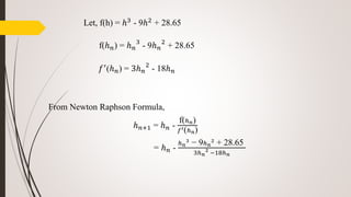
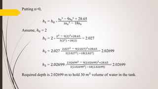
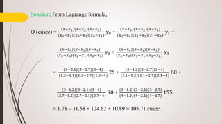
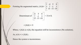
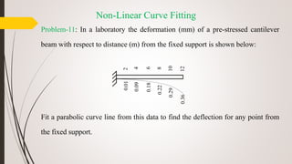
![Problem-4: You are designing a spherical tank to hold water for a small village in a
developing country. The volume of liquid can be calculated as V = πℎ2 [3𝑅−ℎ]
3
. If R = 3
m, to what depth must the tank be filled so that it holds 30 𝑚3 water?
Solution: V = πℎ2 [3𝑅−ℎ]
3
=> 30 = πℎ2 [3.3−ℎ]
3
=> 90 = πℎ2(9-h)
=>
90
𝜋
= 9ℎ2 - ℎ3
=> ℎ3
- 9ℎ2
+ 28.65 = 0](https://image.slidesharecdn.com/ce205-200326191144/85/Numerical-Methods-and-Analysis-17-320.jpg)

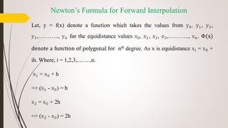
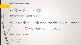
![The polynomial φ(x) = 𝑎0 + 𝑎1 (x-x0) + 𝑎2 (x-x0) (x-x1) + 𝑎3 (x-x0) (x-x1) (x-x2)
+ ………………..+ 𝑎 𝑛 (x-x0) (x-x1) (x-x2)………… (x-x 𝑛−1) ………(1)
When, x = 𝑥0, φ(x) = 𝑎0 = 𝑦0
When, x = 𝑥1, φ(x) = 𝑎0 + 𝑎1 (x1 -x0) = 𝑦1
𝑎1 =
𝑦1−𝑦0
𝑥1−𝑥0
=
∆y0
ℎ
When, x = 𝑥2, φ(x) = 𝑎0 + 𝑎1 (x2 -x0) + 𝑎2 (x2 -x0) (x2 -x1) = 𝑦2
=> 𝑦2 = 𝑦0 +
∆y0
ℎ
. 2h + 𝑎2 . 2h . h [∆y0 = 𝑦1-𝑦0]
=> 𝑎2 =
𝑦2−2𝑦1+ 𝑦0
2ℎ2 =
∆2y0
2!ℎ2](https://image.slidesharecdn.com/ce205-200326191144/85/Numerical-Methods-and-Analysis-24-320.jpg)
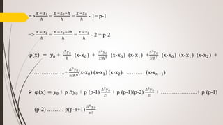


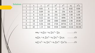
![Problem-12: Use 4 segment to calculate the are of a function f(x) = 0.2 + 25 x +
3𝑥2 + 2𝑥4 from a = 0 to b = 2 by using Trapezoidal rule and Simpson's rule and
determine percentage of error.
Solution: For four segment n = 4. So, the value of x will be 0.5, 1.0, 1.5, 2.0.
Using Trapezoidal rules,
0
2
𝑦𝑑𝑥 =
ℎ
2
[𝑦0+ 𝑦𝑛 + 2 (𝑦1 +……..+ 𝑦(𝑛−1))]
=
0.5
2
[ 0.2 + 94.2 + 2(13.575 + 30.2 + 54.575)] = 72.775 unit
x 0 0.5 1.0 1.5 2.0
y 0.2 13.575 30.2 54.575 94.2](https://image.slidesharecdn.com/ce205-200326191144/85/Numerical-Methods-and-Analysis-55-320.jpg)
![Using Simpson’s rules,
0
2
𝑦𝑑𝑥 =
ℎ
3
[𝑦0+ 𝑦𝑛 + 4 (𝑦1 + 𝑦3 + 𝑦5 +……..+ 𝑦(𝑛−1)) + 2 (𝑦2 + 𝑦4 + 𝑦6 +
……..+ 𝑦(𝑛−2))]
=
0.5
3
[ 0.2 + 94.2 + 4(13.575 + 54.575) + 2 (30.2)] = 71.23 unit
Actual area by integration method,
0
2
𝑦𝑑𝑥 = 0
2
(0.2 + 25 x + 3𝑥2 + 2𝑥4)𝑑𝑥
= 0.2x + 25
𝑥2
2
+ 3
𝑥3
3
+ 2
𝑥5
5 0
2
= 71.2 unit
Percentage of error for Trapezoidal rule =
72.775 −71.2
71.2
x 100% = 2.21%
Percentage of error for Simpson’s rule =
721.23 −71.2
71.2
x 100% = 0.042%](https://image.slidesharecdn.com/ce205-200326191144/85/Numerical-Methods-and-Analysis-56-320.jpg)
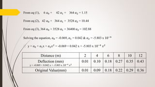
![Problem-13: A irrigation reservoir discharging through sluice at a depth h, below the
water surface as a surface area A, for various value of h as given below:
If t denotes the time in min & the rate of fall of the surface is given by
𝑑ℎ
𝑑𝑡
= -
48
𝐴
ℎ , estimate the time taken for the water level to fall from 14 ft to 10 ft above
the sluice.
Solution: Area of the water reservoir, A =
ℎ
2
[ 950 + 1530 + 2 (1070 + 1200 + 1350)]
= 4860 𝑓𝑡2
h (ft) 10 11 12 13 14
A (𝑓𝑡2
) 950 1070 1200 1350 1530](https://image.slidesharecdn.com/ce205-200326191144/85/Numerical-Methods-and-Analysis-57-320.jpg)
![𝑑ℎ
𝑑𝑡
= -
48
𝐴
ℎ
𝑑ℎ
ℎ
1
2
= -
48
𝐴
dt
10
14
ℎ−1
2 𝑑ℎ = -
48
𝐴 0
𝑡
𝑑𝑡
[
ℎ
1
2
1
2
]
10
14
= -
48
4860
t
t =
4860
48
x
0.58
1
2
= 117.45 min.](https://image.slidesharecdn.com/ce205-200326191144/85/Numerical-Methods-and-Analysis-58-320.jpg)
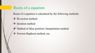
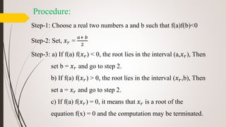
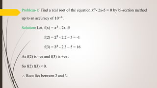
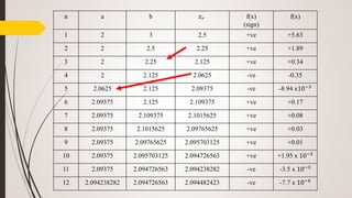
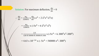
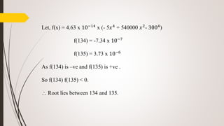
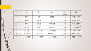
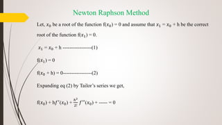
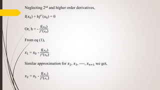
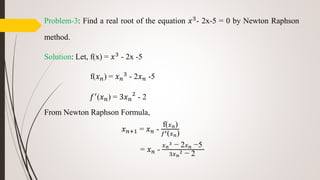
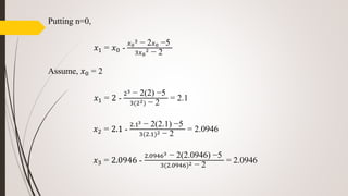
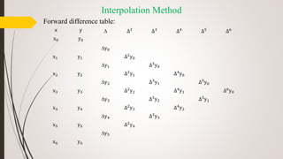
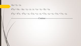
Numerical Methods and Analysis discusses various root-finding methods including bisection, false position, and Newton-Raphson. Bisection uses interval halving to find a root between two values with opposite signs. False position uses the slope of a line between two points to estimate the next root. Newton-Raphson approximates the root using Taylor series expansion neglecting higher order terms. Interpolation uses forward difference tables to construct a polynomial approximation of a function.