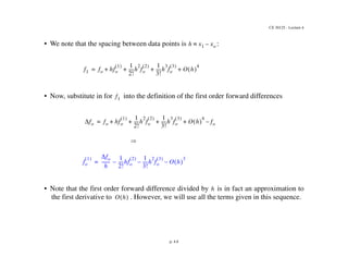
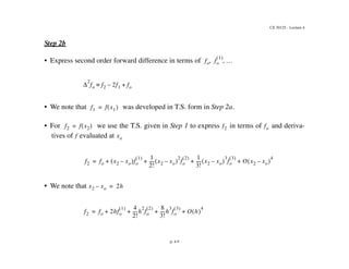
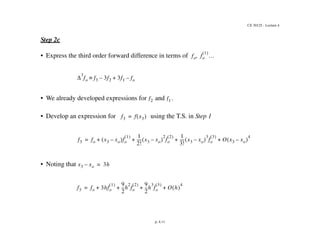
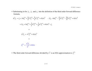
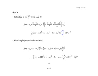
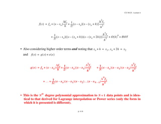
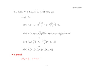
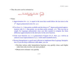
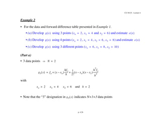
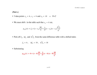
CE 30125 - Lecture 4
p. 4.1
LECTURE 4
NEWTON FORWARD INTERPOLATION ON EQUISPACED POINTS
• Lagrange Interpolation has a number of disadvantages
• The amount of computation required is large
• Interpolation for additional values of requires the same amount of effort as the
first value (i.e. no part of the previous calculation can be used)
• When the number of interpolation points are changed (increased/decreased), the
results of the previous computations can not be used
• Error estimation is difficult (at least may not be convenient)
• Use Newton Interpolation which is based on developing difference tables for a given set
of data points
• The degree interpolating polynomial obtained by fitting data points will be
identical to that obtained using Lagrange formulae!
• Newton interpolation is simply another technique for obtaining the same interpo-
lating polynomial as was obtained using the Lagrange formulae
x
N
th
N 1
+
CE 30125 - Lecture 4
p. 4.2
Forward Difference Tables
• We assume equi-spaced points (not necessary)
• Forward differences are now defined as follows:
(Zeroth
order forward difference)
(First order forward difference)
x0
f1 = f(x1)
f f2 = f(x2)
f3 = f(x3)
f0 = f(x0) fN = f(xN)
x1 x2 x3 xN
x
0 1 2 3
h = interval size
N (i)
0fi fi

fi fi 1
+ fi
–

CE 30125 - Lecture 4
p. 4.3
(Second order forward difference)
(Third order forward difference)
(kth
order forward difference)
• Typically we set up a difference table

2
fi fi 1
+ fi
–


2
fi fi 2
+ fi 1
+
–
  fi 1
+ fi
–
 
–
=

2
fi fi 2
+ 2fi 1
+ fi
+
–
=

3
fi 
2
fi 1
+ 
2
fi
–


3
fi fi 3
+ 2fi 2
+ fi 1
+
+
–
  fi 2
+ 2fi 1
+ fi
+
–
 
–
=

3
fi fi 3
+ 3fi 2
+ 3fi 1
+ fi
–
+
–
=

k
fi 
k 1
–
fi 1
+ 
k 1
–
fi
–
=
CE 30125 - Lecture 4
p. 4.4
• Note that to compute higher order differences in the tables, we take forward differences
of previous order differences instead of using expanded formulae.
• The order of the differences that can be computed depends on how many total data
points, , are available
• data points can develop up to order forward differences
0
1
2
3
4
i fi fi 
2
fi 
3
fi 
4
fi
fo fo f1 fo
–
= 
2
fo f1 fo
–
= 
3
fo 
2
f1 
2
fo
–
= 
4
fo 
3
f1 
3
fo
–
=
f1 f1 f2 f1
–
= 
2
f1 f2 f1
–
= 
3
f1 
2
f2 
2
f1
–
=
f2 f2 f3 f2
–
= 
2
f2 f3 f2
–
=
f3 f3 f4 f3
–
=
f4
xo  xN
 
N 1
+ N
th
CE 30125 - Lecture 4
p. 4.5
Example 1
• Develop a forward difference table for the data given
0 2 -7 4 5 5 3 1
1 4 -3 9 10 8 4
2 6 6 19 18 12
3 8 25 37 30
4 10 62 67
5 12 129
i xi fi fi 
2
fi 
3
fi 
4
fi 
5
fi
CE 30125 - Lecture 4
p. 4.6
Deriving Newton Forward Interpolation on Equi-spaced Points
• Summary of Steps
• Step 1: Develop a general Taylor series expansion for about .
• Step 2: Express the various order forward differences at in terms of and its
derivatives evaluated at . This will allow us to express the actual derivatives eval-
uated at in terms of forward differences.
• Step 3: Using the general Taylor series expansion developed in Step 1, sequentially
substitute in for the derivatives evaluated at in terms of forward differences (i.e.
substitute in the expressions developed in Step 2).
x0
f1
f(x)
f2 f3
f0
fN
x1 x2 x3 xN
x
f x
  xo
xo f x
 
xo
xo
xo
CE 30125 - Lecture 4
p. 4.7
Step 1
• The Taylor series expansion for about is:

Step 2a
• Express first order forward difference in terms of ,
• However since , we can use the Taylor series given in Step 1 to express in
terms of and its derivatives:
f x
  xo
f x
  f xo
  x xo
–
 
df
dx
-----
-
x xo
=
1
2!
----
- x xo
–
 
2 d
2
f
dx
2
-------
-
x xo
=
1
3!
----
- x xo
–
 
3 d
3
f
dx
3
-------
-
x xo
=
O x xo
–
 
4
+
+ + +
=
f x
  fo x xo
–
 fo
1
  1
2!
----
- x xo
–
 
2
fo
2
  1
3!
----
- x xo
–
 
3
fo
3
 
O x xo
–
 
4
+ + + +
=
fo fo
1
 


fo f1 fo
–

f1 f x1
 
= f1
fo
f1 fo x1 xo
–
 fo
1
  1
2!
----
- x1 xo
–
 
2
fo
2
  1
3!
----
- x1 xo
–
 
3
fo
3
 
O x1 xo
–
 
4
+ + + +
=
CE 30125 - Lecture 4
p. 4.8
• We note that the spacing between data points is :
• Now, substitute in for into the definition of the first order forward differences

• Note that the first order forward difference divided by is in fact an approximation to
the first derivative to . However, we will use all the terms given in this sequence.
h x1 xo
–

f1 fo hfo
1
  1
2!
----
-h
2
fo
2
  1
3!
----
-h
3
fo
3
 
O h
 
4
+ + + +
=
f1
fo fo hfo
1
  1
2!
----
-h
2
fo
2
  1
3!
----
-h
3
fo
3
 
O h
 
4
fo
–
+ + + +
=
fo
1
  fo
h
-------
-
1
2!
----
-
– hfo
2
  1
3!
----
-h
2
fo
3
 
O h
 
3
–
–
=
h
O h
 
CE 30125 - Lecture 4
p. 4.9
Step 2b
• Express second order forward difference in terms of
• We note that was developed in T.S. form in Step 2a.
• For we use the T.S. given in Step 1 to express in terms of and deriva-
tives of evaluated at
• We note that
fo fo
1
 

 

2
fo f2 2f1 fo
+
–

f1 f x1
 
=
f2 f x2
 
= f2 fo
f xo
f2 fo x2 xo
–
 fo
1
  1
2!
----
- x2 xo
–
 
2
fo
2
  1
3!
----
- x2 xo
–
 
3
fo
3
 
O x2 xo
–
 
4
+ + + +
=
x2 xo
– 2h
=
f2 fo 2hfo
1
  4
2!
----
-h
2
fo
2
  8
3!
----
-h
3
fo
3
 
O h
 
4
+ + + +
=
CE 30125 - Lecture 4
p. 4.10
• Now substitute in for and into the definition of the second order forward difference
operator

• Note that the second order forward difference divided by is in fact an approximation
to to . However, we will use all terms in the expression.
f2 f1

2
fo fo 2hfo
1
 
2h
2
fo
2
  4
3
--
-h
3
fo
3
 
O h
 
4
+ + + +
= 2fo
– 2hfo
1
 
h
2
fo
2
  1
3
--
-h
3
fo
3
 
O h
 
4
fo
+ +
–
–
–
fo
2
  
2
fo
h
2
---------
- hfo
3
 
O h
 
2
+
–
=
h
2
fo
2
 
O h
 
CE 30125 - Lecture 4
p. 4.11
Step 2c
• Express the third order forward difference in terms of
• We already developed expressions for and .
• Develop an expression for using the T.S. in Step 1
• Noting that
fo fo
1
 



3
fo f3 3f2 3f1
+
– fo
–

f2 f1
f3 f x3
 
=
f3 fo x3 xo
–
 fo
1
  1
2!
----
- x3 xo
–
 
2
fo
2
  1
3!
----
- x3 xo
–
 
3
fo
3
 
O x3 xo
–
 
4
+ + + +
=
x3 xo
– 3h
=
f3 fo 3hfo
1
  9
2
--
-h
2
fo
2
  9
2
--
-h
3
fo
3
 
O h
 
4
+ + + +
=
CE 30125 - Lecture 4
p. 4.12
• Substituting in for , and into the definition of the third order forward difference
formula.


• The third order forward difference divided by is an O(h) approximation to
f3 f2 f1

3
fo fo 3hfo
1
  9
2
--
-h
2
fo
2
  9
2
--
-h
3
fo
3
 
O h
 
4
+ + + +
= 3fo
– 6hfo
1
 
–
12
2
-----
-h
2
fo
2
 
–
24
3!
-----
-h
3
fo
3
 
– O h
 
4
+
3fo 3hfo
1
  3
2
--
-h
2
fo
2
  3
3!
----
-h
3
fo
3
 
O h
 
4
fo
–
+ + + + +

3
fo h
3
fo
3
 
O h
 
4
+
=
fo
3
  
3
fo
h
3
---------
- O h
 
+
=
h
3
fo
3
 
CE 30125 - Lecture 4
p. 4.13
Step 3a
• Consider the general T.S. expansion presented in Step 1 to define and substitute in
for using the result in Step 2a.
• Note that now we are not evaluating the T.S. at a data point but at any

f x
 
fo
1
 
x
f x
  fo x xo
–
 
+
fo
h
-------
-
1
2!
----
-hfo
2
  1
3!
----
-h
2
fo
3
 
O h
 
3
–
–
–
=
1
2!
----
- x xo
–
 
2
fo
2
  1
3!
----
- x xo
–
 
3
fo
3
 
O x xo
–
 
4
+ + +
f x
  fo
x xo
–
h
------------
-fo
1
2!
----
- x xo
–
 h
– x xo
–
 
2
+
 fo
2
 
+ +
=
1
3!
----
- x xo
–
 h
2
– x xo
–
 
3
+
 fo
3
 
O h
 
4
+ +
CE 30125 - Lecture 4
p. 4.14
Step 3b
• Substitute in for using the expression developed in Step 2b.

fo
2
 
f x
  fo
x xo
–
h
-------------fo
1
2!
----
- x xo
–
 h
– x xo
–
 
2
+
 

2
fo
h
2
---------
- hfo
3
 
O h
 
2
+
–
+ +
=
1
3!
----
- x xo
–
 
– h
2
x xo
–
 
3
+
 fo
3
 
O h
 
4
+
+
f x
  fo
x xo
–
h
-------------fo
1
2!
----
-
x xo
–
 
h
-----------------
-
–
x xo
–
 
2
h
2
--------------------
-
+ 
2
fo
+ +
=
1
3!
----
- 2 x xo
–
 h
2
x xo
–
 
3
3 x xo
–
 
2
h
–
+
 
+ fo
3
 
O h
 
4
+
CE 30125 - Lecture 4
p. 4.15
Step 3c
• Substitute in for from Step 2c
• Re-arranging the terms in brackets:

fo
3
 
f x
  fo
x xo
–
 
h
-----------------
-fo
1
2!
----
-
x xo
–
 
h
-----------------
-
–
x xo
–
 
2
h
2
--------------------
-
+ 
2
fo
+ +
=
1
3!
----
- 2 x xo
–
 h
2
x xo
–
 
3
3 x xo
–
 
2
h
–
+
 

3
fo
h
3
---------
- O h
 
4
+ +
f x
  fo x xo
–
 
fo
h
-------
-
1
2!
----
- x xo
–
 
+ + h
– x xo
–
 
+
 

2
fo
h
2
---------
-
=
1
3!
----
- x xo
–
  2h
2
x xo
–
 
2
3 x xo
–
 h
–
+
 

3
fo
h
3
---------
- O h
 
4
HOT
+ + +
CE 30125 - Lecture 4
p. 4.16
• Also considering higher order terms and noting that ,
and
• This is the degree polynomial approximation to data points and is iden-
tical to that derived for Lagrange interpolation or Power series (only the form in
which it is presented is different).
f x
  fo x xo
–
 
fo
h
-------
-
1
2!
----
- x xo
–
  x xo h
+
 
–
 

2
fo
h
2
---------
-
+ +
=
1
3!
----
- x xo
–
  x xo h
+
 
–
  x xo 2h
+
 
–
 
 

3
fo
h
3
---------
- O h
 
4
HOT
+ + +
xo h
+ x1
= xo 2h
+ x2
=
f x
  g x
  e x
 
+
=
g x
  fo x xo
–
 
fo
h
-------
-
1
2!
----
- x xo
–
  x x1
–
 

2
fo
h
2
----------
+ +
=
1
3!
----
- x xo
–
  x x1
–
  x x2
–
 

3
fo
h
3
----------
+

1
N!
-----
-
+ + x xo
–
  x x1
–
  x x2
–
  x xN 1
–
–
 

N
fo
h
N
-----------
N
th
N 1
+
CE 30125 - Lecture 4
p. 4.17
• Note that the data point are exactly fit by


• In general
N 1
+ g x
 
g xo
  fo
=
g x1
  fo x1 xo
–
 
f1 fo
–
h
-------------
-
+ fo h
f1 fo
–
h
-------------
-
 
 
+ f1
= = =
g x2
  fo x2 xo
–
 
f1 fo
–
h
-------------
-
 
  1
2
--
- x2 xo
–
  x2 x1
–
 
1
h
2
----
- f2 2f1 fo
+
–
 
+ +
=
g x2
  fo
2h
h
-----
- f1 fo
–
 
2h
 h
2h
2
-------------
- f2 2f1 fo
+
–
 
+ +
=
g x2
  fo 2f1 2fo
– f2 2f1
– fo
+ + + f2
= =
g xi
  fi
= i 0 N

=
CE 30125 - Lecture 4
p. 4.18
• It can be readily shown that the error at any is: (by carrying through error terms in the
T.S.)
• This error function is identical to that for Lagrange Interpolation (since the polynomial
approximation is the same).
• However we note that can be approximated as (can be shown by T.S.)
• In fact if does not vary dramatically over the interval
x
e x
  f x
  g x
 
–
x xo
–
  x x1
–
  x xN
–
 
N 1
+
 !
-----------------------------------------------------------------
-f
N 1
+
 

 
= = xo  xN
 
f
N 1
+
x
 
f
N 1
+
 
xo
 

N 1
+
fo
h
N 1
+
-----------------
-

f
N 1
+
 
x
 
f
N 1
+
 

 

N 1
+
fo
h
N 1
+
-----------------
-

CE 30125 - Lecture 4
p. 4.19
• Thus the error can be estimated as
• Notes
• Approximation for is equal to the term that would follow the last term in the
degree polynomial series for
• If we have data points available and develop an degree polynomial approx-
imation with data points, we can then easily estimate . This was not as
simple for Lagrange polynomials since you then needed to compute the finite
difference approximation to the derivative in the error function.
• If the exact function is a polynomial of degree , then will be an
(almost) exact representation of (with small roundoff errors).
• Newton Interpolation is much more efficient to implement than Lagrange Interpola-
tion. If you develop a difference table once, you can
• Develop various order interpolation functions very quickly (since each higher
order term only involves one more product)
• Obtain error estimates very quickly
e x
 
x xo
–
  x x1
–
  x xN
–
 
N 1
+
 !
-----------------------------------------------------------------
-

N 1
+
fo
h
N 1
+
------------------
-

e x
 
N
th
g x
 
N 2
+ N
th
N 1
+ e x
 
f x
  M N
 g x
 
f x
 
CE 30125 - Lecture 4
p. 4.20
Example 2
• For the data and forward difference table presented in Example 1.
• (a) Develop using 3 points ( , and ) and estimate
• (b) Develop using 4 points ( , , , ) and estimate
• (c) Develop using 3 different points ( , , )
(Part a)
• 3 data points 
with
and
• Note that the “3” designation in indicates N+1=3 data points
g x
  xo 2
= x1 4
= x2 6
= e x
 
g x
  xo 2
= x1 4
= x2 6
= x3 8
= e x
 
g x
  xo 6
= x1 8
= x2 10
=
N 2
=
g3 x
  fo x xo
–
 
fo
h
-------
-
1
2!
----
- x xo
–
  x x1
–
 

2
fo
h
2
---------
-
+ +
=
xo 2
= x1 4
= x2 6
= h 2
=
g3 x
 
CE 30125 - Lecture 4
p. 4.21
• , and are obtained by simply picking values off of the difference table
(across the row )
• The error can be estimated as:
• Simply substitute in for , , , and pick off = 5 from the table in Example 1
fo fo 
2
fo
i 0
=
fo 7
–
= fo 4
= 
2
fo 5
=
g3 x
  7
– x 2
–
 
4
2
--
-
1
2!
----
- x 2
–
  x 4
–
 
5
4
--
-
+ +
=
e3 x
 
x xo
–
  x x1
–
  x x2
–
 
3!
-------------------------------------------------------
-
1
h
3
----
-
3
fo
=
xo x1 x2 h 
3
fo
e3 x
 
x 2
–
  x 4
–
  x 6
–
 
6
--------------------------------------------------
-
1
2
3
----
- 5
  x 2
–
  x 4
–
  x 6
–
 
5
48
-----
-
= =
CE 30125 - Lecture 4
p. 4.22
(Part b)
• 4 data points , , , 
• Simply add the next term to the series for in Part a:
• We note that the term we are adding to is actually
• Pick off = 5 from the table in Example 1 and substitute in
• The error is estimated as

xo 2
= x1 4
= x2 6
= x3 8
= N 3
=
g3 x
 
g4 x
  g3 x
 
1
3!
----
- x xo
–
  x x1
–
  x x2
–
 

3
fo
h
3
---------
-
+
=
g3 x
  e3 x
 

3
fo
g4 x
  g3 x
 
1
3!
----
- x 2
–
  x 4
–
  x 6
–
 
+
5
8
--
-

=
e4 x
 
x xo
–
  x x1
–
  x x2
–
  x x3
–
 
4!
--------------------------------------------------------------------------
-
1
h
4
----
-
4
fo
=
e4 x
  x 2
–
  x 4
–
  x 6
–
  x 8
–
 
3
384
--------
-
=
CE 30125 - Lecture 4
p. 4.23
(Part c)
• 3 data points , and N=2
• We must shift in the table such that etc.
• Pick off , and from the same difference table with a shifted index
, ,
• Substituting
xo 6
= x1 8
= x3 10
=
i xo 6
=
g3/s x
  fo x xo
–
 
fo
h
-------
-
1
2!
----
- x xo
–
  x x1
–
 

2
fo
h
2
---------
-
+ +
=
fo fo 
2
fo
fo 6
= fo 19
= 
2
fo 18
=
g3/s x
  6 x 6
–
 
19
2
-----
-
1
2!
----
- x 6
–
  x 8
–
 
18
2
2
-----
-
+ +
=
CE 30125 - Lecture 4
p. 4.24
Newton Backward Interpolation
• Newton backward interpolation is essentially the same as Newton forward interpolation
except that backward differences are used
• Backward differences are defined as:
Zeroth order backward difference
First order backward difference
Second order backward difference
kth
order backward difference

o
fi fi

fi fi fi 1
–
–
=

2
fi fi fi 1
–
–
=

k
fi 
k 1
–
fi 
k 1
–
fi 1
–
–
=
CE 30125 - Lecture 4
p. 4.25
• For data point which are fitted with an degree polynomial
• Note that we are really expanding about the right most point to the left. Therefore we
must develop , etc. in the difference table
N 1
+ N
th
g x
  fN x xN
–
 
fN
h
---------
-
1
2!
----
-
+ + x xN
–
  x xN 1
–
–
 

2
fN
h
2
-----------
-
=
1
3!
----
-
+ x xN
–
  x xN 1
–
–
  x xN 2
–
–
 

3
fN
h
3
-----------
-
1
N!
-----
-
+ x xN
–
  x xN 1
–
–
  x x1
–
 

N
fN
h
N
------------
-
fN fN
xN
x0 x1
xN - 1
CE 30125 - Lecture 4
p. 4.26
Newton Interpolation on Non-uniformly Spaced Data Points
• Newton interpolation can be readily extended to deal with non-uniformly spaced data
points
• The difference table for non-uniformly spaced nodes is developed and an appropriate
interpolation formula is developed and used
x0 x1 x2 x3 x4
x
CE 30125 - Lecture 4
p. 4.27
SUMMARY OF LECTURE 4
• Newton formulae can be obtained by manipulating Taylor series
• Newton interpolating function is related to easily computed forward/backward differ-
ences
• Error is readily established and estimated from the difference table (as long as you have
one more data point than used in interpolation)
• Newton interpolation through data points gives the same degree polynomial as
Lagrange interpolation
• Newton interpolation is more efficient than Lagrange interpolation and is easily imple-
mented
N 1
+ N
th

Engineering mathematics module 3 civil engineering

  • 1.
    CE 30125 -Lecture 4 p. 4.1 LECTURE 4 NEWTON FORWARD INTERPOLATION ON EQUISPACED POINTS • Lagrange Interpolation has a number of disadvantages • The amount of computation required is large • Interpolation for additional values of requires the same amount of effort as the first value (i.e. no part of the previous calculation can be used) • When the number of interpolation points are changed (increased/decreased), the results of the previous computations can not be used • Error estimation is difficult (at least may not be convenient) • Use Newton Interpolation which is based on developing difference tables for a given set of data points • The degree interpolating polynomial obtained by fitting data points will be identical to that obtained using Lagrange formulae! • Newton interpolation is simply another technique for obtaining the same interpo- lating polynomial as was obtained using the Lagrange formulae x N th N 1 +
  • 2.
    CE 30125 -Lecture 4 p. 4.2 Forward Difference Tables • We assume equi-spaced points (not necessary) • Forward differences are now defined as follows: (Zeroth order forward difference) (First order forward difference) x0 f1 = f(x1) f f2 = f(x2) f3 = f(x3) f0 = f(x0) fN = f(xN) x1 x2 x3 xN x 0 1 2 3 h = interval size N (i) 0fi fi  fi fi 1 + fi – 
  • 3.
    CE 30125 -Lecture 4 p. 4.3 (Second order forward difference) (Third order forward difference) (kth order forward difference) • Typically we set up a difference table  2 fi fi 1 + fi –   2 fi fi 2 + fi 1 + –   fi 1 + fi –   – =  2 fi fi 2 + 2fi 1 + fi + – =  3 fi  2 fi 1 +  2 fi –   3 fi fi 3 + 2fi 2 + fi 1 + + –   fi 2 + 2fi 1 + fi + –   – =  3 fi fi 3 + 3fi 2 + 3fi 1 + fi – + – =  k fi  k 1 – fi 1 +  k 1 – fi – =
  • 4.
    CE 30125 -Lecture 4 p. 4.4 • Note that to compute higher order differences in the tables, we take forward differences of previous order differences instead of using expanded formulae. • The order of the differences that can be computed depends on how many total data points, , are available • data points can develop up to order forward differences 0 1 2 3 4 i fi fi  2 fi  3 fi  4 fi fo fo f1 fo – =  2 fo f1 fo – =  3 fo  2 f1  2 fo – =  4 fo  3 f1  3 fo – = f1 f1 f2 f1 – =  2 f1 f2 f1 – =  3 f1  2 f2  2 f1 – = f2 f2 f3 f2 – =  2 f2 f3 f2 – = f3 f3 f4 f3 – = f4 xo  xN   N 1 + N th
  • 5.
    CE 30125 -Lecture 4 p. 4.5 Example 1 • Develop a forward difference table for the data given 0 2 -7 4 5 5 3 1 1 4 -3 9 10 8 4 2 6 6 19 18 12 3 8 25 37 30 4 10 62 67 5 12 129 i xi fi fi  2 fi  3 fi  4 fi  5 fi
  • 6.
    CE 30125 -Lecture 4 p. 4.6 Deriving Newton Forward Interpolation on Equi-spaced Points • Summary of Steps • Step 1: Develop a general Taylor series expansion for about . • Step 2: Express the various order forward differences at in terms of and its derivatives evaluated at . This will allow us to express the actual derivatives eval- uated at in terms of forward differences. • Step 3: Using the general Taylor series expansion developed in Step 1, sequentially substitute in for the derivatives evaluated at in terms of forward differences (i.e. substitute in the expressions developed in Step 2). x0 f1 f(x) f2 f3 f0 fN x1 x2 x3 xN x f x   xo xo f x   xo xo xo
  • 7.
    CE 30125 -Lecture 4 p. 4.7 Step 1 • The Taylor series expansion for about is:  Step 2a • Express first order forward difference in terms of , • However since , we can use the Taylor series given in Step 1 to express in terms of and its derivatives: f x   xo f x   f xo   x xo –   df dx ----- - x xo = 1 2! ---- - x xo –   2 d 2 f dx 2 ------- - x xo = 1 3! ---- - x xo –   3 d 3 f dx 3 ------- - x xo = O x xo –   4 + + + + = f x   fo x xo –  fo 1   1 2! ---- - x xo –   2 fo 2   1 3! ---- - x xo –   3 fo 3   O x xo –   4 + + + + = fo fo 1     fo f1 fo –  f1 f x1   = f1 fo f1 fo x1 xo –  fo 1   1 2! ---- - x1 xo –   2 fo 2   1 3! ---- - x1 xo –   3 fo 3   O x1 xo –   4 + + + + =
  • 8.
    CE 30125 -Lecture 4 p. 4.8 • We note that the spacing between data points is : • Now, substitute in for into the definition of the first order forward differences  • Note that the first order forward difference divided by is in fact an approximation to the first derivative to . However, we will use all the terms given in this sequence. h x1 xo –  f1 fo hfo 1   1 2! ---- -h 2 fo 2   1 3! ---- -h 3 fo 3   O h   4 + + + + = f1 fo fo hfo 1   1 2! ---- -h 2 fo 2   1 3! ---- -h 3 fo 3   O h   4 fo – + + + + = fo 1   fo h ------- - 1 2! ---- - – hfo 2   1 3! ---- -h 2 fo 3   O h   3 – – = h O h  
  • 9.
    CE 30125 -Lecture 4 p. 4.9 Step 2b • Express second order forward difference in terms of • We note that was developed in T.S. form in Step 2a. • For we use the T.S. given in Step 1 to express in terms of and deriva- tives of evaluated at • We note that fo fo 1       2 fo f2 2f1 fo + –  f1 f x1   = f2 f x2   = f2 fo f xo f2 fo x2 xo –  fo 1   1 2! ---- - x2 xo –   2 fo 2   1 3! ---- - x2 xo –   3 fo 3   O x2 xo –   4 + + + + = x2 xo – 2h = f2 fo 2hfo 1   4 2! ---- -h 2 fo 2   8 3! ---- -h 3 fo 3   O h   4 + + + + =
  • 10.
    CE 30125 -Lecture 4 p. 4.10 • Now substitute in for and into the definition of the second order forward difference operator  • Note that the second order forward difference divided by is in fact an approximation to to . However, we will use all terms in the expression. f2 f1  2 fo fo 2hfo 1   2h 2 fo 2   4 3 -- -h 3 fo 3   O h   4 + + + + = 2fo – 2hfo 1   h 2 fo 2   1 3 -- -h 3 fo 3   O h   4 fo + + – – – fo 2    2 fo h 2 --------- - hfo 3   O h   2 + – = h 2 fo 2   O h  
  • 11.
    CE 30125 -Lecture 4 p. 4.11 Step 2c • Express the third order forward difference in terms of • We already developed expressions for and . • Develop an expression for using the T.S. in Step 1 • Noting that fo fo 1      3 fo f3 3f2 3f1 + – fo –  f2 f1 f3 f x3   = f3 fo x3 xo –  fo 1   1 2! ---- - x3 xo –   2 fo 2   1 3! ---- - x3 xo –   3 fo 3   O x3 xo –   4 + + + + = x3 xo – 3h = f3 fo 3hfo 1   9 2 -- -h 2 fo 2   9 2 -- -h 3 fo 3   O h   4 + + + + =
  • 12.
    CE 30125 -Lecture 4 p. 4.12 • Substituting in for , and into the definition of the third order forward difference formula.   • The third order forward difference divided by is an O(h) approximation to f3 f2 f1  3 fo fo 3hfo 1   9 2 -- -h 2 fo 2   9 2 -- -h 3 fo 3   O h   4 + + + + = 3fo – 6hfo 1   – 12 2 ----- -h 2 fo 2   – 24 3! ----- -h 3 fo 3   – O h   4 + 3fo 3hfo 1   3 2 -- -h 2 fo 2   3 3! ---- -h 3 fo 3   O h   4 fo – + + + + +  3 fo h 3 fo 3   O h   4 + = fo 3    3 fo h 3 --------- - O h   + = h 3 fo 3  
  • 13.
    CE 30125 -Lecture 4 p. 4.13 Step 3a • Consider the general T.S. expansion presented in Step 1 to define and substitute in for using the result in Step 2a. • Note that now we are not evaluating the T.S. at a data point but at any  f x   fo 1   x f x   fo x xo –   + fo h ------- - 1 2! ---- -hfo 2   1 3! ---- -h 2 fo 3   O h   3 – – – = 1 2! ---- - x xo –   2 fo 2   1 3! ---- - x xo –   3 fo 3   O x xo –   4 + + + f x   fo x xo – h ------------ -fo 1 2! ---- - x xo –  h – x xo –   2 +  fo 2   + + = 1 3! ---- - x xo –  h 2 – x xo –   3 +  fo 3   O h   4 + +
  • 14.
    CE 30125 -Lecture 4 p. 4.14 Step 3b • Substitute in for using the expression developed in Step 2b.  fo 2   f x   fo x xo – h -------------fo 1 2! ---- - x xo –  h – x xo –   2 +    2 fo h 2 --------- - hfo 3   O h   2 + – + + = 1 3! ---- - x xo –   – h 2 x xo –   3 +  fo 3   O h   4 + + f x   fo x xo – h -------------fo 1 2! ---- - x xo –   h ----------------- - – x xo –   2 h 2 -------------------- - +  2 fo + + = 1 3! ---- - 2 x xo –  h 2 x xo –   3 3 x xo –   2 h – +   + fo 3   O h   4 +
  • 15.
    CE 30125 -Lecture 4 p. 4.15 Step 3c • Substitute in for from Step 2c • Re-arranging the terms in brackets:  fo 3   f x   fo x xo –   h ----------------- -fo 1 2! ---- - x xo –   h ----------------- - – x xo –   2 h 2 -------------------- - +  2 fo + + = 1 3! ---- - 2 x xo –  h 2 x xo –   3 3 x xo –   2 h – +    3 fo h 3 --------- - O h   4 + + f x   fo x xo –   fo h ------- - 1 2! ---- - x xo –   + + h – x xo –   +    2 fo h 2 --------- - = 1 3! ---- - x xo –   2h 2 x xo –   2 3 x xo –  h – +    3 fo h 3 --------- - O h   4 HOT + + +
  • 16.
    CE 30125 -Lecture 4 p. 4.16 • Also considering higher order terms and noting that , and • This is the degree polynomial approximation to data points and is iden- tical to that derived for Lagrange interpolation or Power series (only the form in which it is presented is different). f x   fo x xo –   fo h ------- - 1 2! ---- - x xo –   x xo h +   –    2 fo h 2 --------- - + + = 1 3! ---- - x xo –   x xo h +   –   x xo 2h +   –      3 fo h 3 --------- - O h   4 HOT + + + xo h + x1 = xo 2h + x2 = f x   g x   e x   + = g x   fo x xo –   fo h ------- - 1 2! ---- - x xo –   x x1 –    2 fo h 2 ---------- + + = 1 3! ---- - x xo –   x x1 –   x x2 –    3 fo h 3 ---------- +  1 N! ----- - + + x xo –   x x1 –   x x2 –   x xN 1 – –    N fo h N ----------- N th N 1 +
  • 17.
    CE 30125 -Lecture 4 p. 4.17 • Note that the data point are exactly fit by   • In general N 1 + g x   g xo   fo = g x1   fo x1 xo –   f1 fo – h ------------- - + fo h f1 fo – h ------------- -     + f1 = = = g x2   fo x2 xo –   f1 fo – h ------------- -     1 2 -- - x2 xo –   x2 x1 –   1 h 2 ---- - f2 2f1 fo + –   + + = g x2   fo 2h h ----- - f1 fo –   2h  h 2h 2 ------------- - f2 2f1 fo + –   + + = g x2   fo 2f1 2fo – f2 2f1 – fo + + + f2 = = g xi   fi = i 0 N  =
  • 18.
    CE 30125 -Lecture 4 p. 4.18 • It can be readily shown that the error at any is: (by carrying through error terms in the T.S.) • This error function is identical to that for Lagrange Interpolation (since the polynomial approximation is the same). • However we note that can be approximated as (can be shown by T.S.) • In fact if does not vary dramatically over the interval x e x   f x   g x   – x xo –   x x1 –   x xN –   N 1 +  ! ----------------------------------------------------------------- -f N 1 +      = = xo  xN   f N 1 + x   f N 1 +   xo    N 1 + fo h N 1 + ----------------- -  f N 1 +   x   f N 1 +       N 1 + fo h N 1 + ----------------- - 
  • 19.
    CE 30125 -Lecture 4 p. 4.19 • Thus the error can be estimated as • Notes • Approximation for is equal to the term that would follow the last term in the degree polynomial series for • If we have data points available and develop an degree polynomial approx- imation with data points, we can then easily estimate . This was not as simple for Lagrange polynomials since you then needed to compute the finite difference approximation to the derivative in the error function. • If the exact function is a polynomial of degree , then will be an (almost) exact representation of (with small roundoff errors). • Newton Interpolation is much more efficient to implement than Lagrange Interpola- tion. If you develop a difference table once, you can • Develop various order interpolation functions very quickly (since each higher order term only involves one more product) • Obtain error estimates very quickly e x   x xo –   x x1 –   x xN –   N 1 +  ! ----------------------------------------------------------------- -  N 1 + fo h N 1 + ------------------ -  e x   N th g x   N 2 + N th N 1 + e x   f x   M N  g x   f x  
  • 20.
    CE 30125 -Lecture 4 p. 4.20 Example 2 • For the data and forward difference table presented in Example 1. • (a) Develop using 3 points ( , and ) and estimate • (b) Develop using 4 points ( , , , ) and estimate • (c) Develop using 3 different points ( , , ) (Part a) • 3 data points  with and • Note that the “3” designation in indicates N+1=3 data points g x   xo 2 = x1 4 = x2 6 = e x   g x   xo 2 = x1 4 = x2 6 = x3 8 = e x   g x   xo 6 = x1 8 = x2 10 = N 2 = g3 x   fo x xo –   fo h ------- - 1 2! ---- - x xo –   x x1 –    2 fo h 2 --------- - + + = xo 2 = x1 4 = x2 6 = h 2 = g3 x  
  • 21.
    CE 30125 -Lecture 4 p. 4.21 • , and are obtained by simply picking values off of the difference table (across the row ) • The error can be estimated as: • Simply substitute in for , , , and pick off = 5 from the table in Example 1 fo fo  2 fo i 0 = fo 7 – = fo 4 =  2 fo 5 = g3 x   7 – x 2 –   4 2 -- - 1 2! ---- - x 2 –   x 4 –   5 4 -- - + + = e3 x   x xo –   x x1 –   x x2 –   3! ------------------------------------------------------- - 1 h 3 ---- - 3 fo = xo x1 x2 h  3 fo e3 x   x 2 –   x 4 –   x 6 –   6 -------------------------------------------------- - 1 2 3 ---- - 5   x 2 –   x 4 –   x 6 –   5 48 ----- - = =
  • 22.
    CE 30125 -Lecture 4 p. 4.22 (Part b) • 4 data points , , ,  • Simply add the next term to the series for in Part a: • We note that the term we are adding to is actually • Pick off = 5 from the table in Example 1 and substitute in • The error is estimated as  xo 2 = x1 4 = x2 6 = x3 8 = N 3 = g3 x   g4 x   g3 x   1 3! ---- - x xo –   x x1 –   x x2 –    3 fo h 3 --------- - + = g3 x   e3 x    3 fo g4 x   g3 x   1 3! ---- - x 2 –   x 4 –   x 6 –   + 5 8 -- -  = e4 x   x xo –   x x1 –   x x2 –   x x3 –   4! -------------------------------------------------------------------------- - 1 h 4 ---- - 4 fo = e4 x   x 2 –   x 4 –   x 6 –   x 8 –   3 384 -------- - =
  • 23.
    CE 30125 -Lecture 4 p. 4.23 (Part c) • 3 data points , and N=2 • We must shift in the table such that etc. • Pick off , and from the same difference table with a shifted index , , • Substituting xo 6 = x1 8 = x3 10 = i xo 6 = g3/s x   fo x xo –   fo h ------- - 1 2! ---- - x xo –   x x1 –    2 fo h 2 --------- - + + = fo fo  2 fo fo 6 = fo 19 =  2 fo 18 = g3/s x   6 x 6 –   19 2 ----- - 1 2! ---- - x 6 –   x 8 –   18 2 2 ----- - + + =
  • 24.
    CE 30125 -Lecture 4 p. 4.24 Newton Backward Interpolation • Newton backward interpolation is essentially the same as Newton forward interpolation except that backward differences are used • Backward differences are defined as: Zeroth order backward difference First order backward difference Second order backward difference kth order backward difference  o fi fi  fi fi fi 1 – – =  2 fi fi fi 1 – – =  k fi  k 1 – fi  k 1 – fi 1 – – =
  • 25.
    CE 30125 -Lecture 4 p. 4.25 • For data point which are fitted with an degree polynomial • Note that we are really expanding about the right most point to the left. Therefore we must develop , etc. in the difference table N 1 + N th g x   fN x xN –   fN h --------- - 1 2! ---- - + + x xN –   x xN 1 – –    2 fN h 2 ----------- - = 1 3! ---- - + x xN –   x xN 1 – –   x xN 2 – –    3 fN h 3 ----------- - 1 N! ----- - + x xN –   x xN 1 – –   x x1 –    N fN h N ------------ - fN fN xN x0 x1 xN - 1
  • 26.
    CE 30125 -Lecture 4 p. 4.26 Newton Interpolation on Non-uniformly Spaced Data Points • Newton interpolation can be readily extended to deal with non-uniformly spaced data points • The difference table for non-uniformly spaced nodes is developed and an appropriate interpolation formula is developed and used x0 x1 x2 x3 x4 x
  • 27.
    CE 30125 -Lecture 4 p. 4.27 SUMMARY OF LECTURE 4 • Newton formulae can be obtained by manipulating Taylor series • Newton interpolating function is related to easily computed forward/backward differ- ences • Error is readily established and estimated from the difference table (as long as you have one more data point than used in interpolation) • Newton interpolation through data points gives the same degree polynomial as Lagrange interpolation • Newton interpolation is more efficient than Lagrange interpolation and is easily imple- mented N 1 + N th