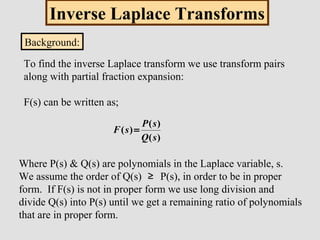
The document discusses the inverse Laplace transform and related topics. It provides three main cases for performing partial fraction expansions when taking the inverse Laplace transform: 1) non-repeated simple roots, 2) complex poles, and 3) repeated poles. It also discusses the convolution integral and how it relates the time domain convolution of two functions to the multiplication of their Laplace transforms. An example uses the convolution integral to find the output of a system given its impulse response and input.

1. The Inverse Laplace Transform
The University of Tennessee
Electrical and Computer Engineering Department
Knoxville, Tennessee
wlg

2. Inverse Laplace Transforms
Background:
To find the inverse Laplace transform we use transform pairs
along with partial fraction expansion:
F(s) can be written as;
)(
)(
)(
sQ
sP
sF =
Where P(s) & Q(s) are polynomials in the Laplace variable, s.
We assume the order of Q(s) P(s), in order to be in proper
form. If F(s) is not in proper form we use long division and
divide Q(s) into P(s) until we get a remaining ratio of polynomials
that are in proper form.
≥

3. Inverse Laplace Transforms
Background:
There are three cases to consider in doing the partial fraction expansion of F(s).
Case 1: F(s) has all non repeated simple roots.
n
n
ps
k
ps
k
ps
k
sF
+
++
+
+
+
= ...)(
2
2
1
1
Case 2: F(s) has complex poles:
++
++
+
−+
=
++−+
= ...
)))()((
)(
)(
*
11
1
1
βαβαβαβα js
k
js
k
jsjssQ
sP
sF
Case 3: F(s) has repeated poles.
)(
)(
...
)(
...
)())((
)(
)(
1
1
1
1
2
1
12
1
11
11
1
sQ
sP
ps
k
ps
k
ps
k
pssQ
sP
sF r
r
r
++
+
++
+
+
+
=
+
= (expanded)
(expanded)

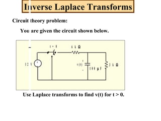
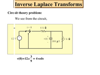
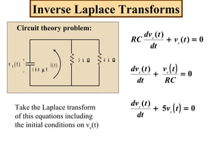
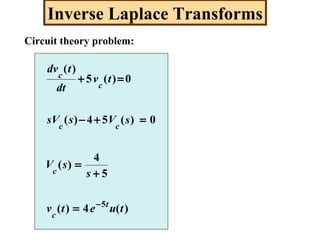
4. Inverse Laplace Transforms
Case 1: Illustration:
Given:
)10()4()1()10)(4)(1(
)2(4
)( 321
+
+
+
+
+
=
+++
+
=
s
A
s
A
s
A
sss
s
sF
274
)10)(4)(1(
)2(4)1(
| 11
=
+++
++
= −=s
sss
ss
A 94
)10)(4)(1(
)2(4)4(
| 42
=
+++
++
= −=ssss
ss
A
2716
)10)(4)(1(
)2(4)10(
| 103
−=
+++
++
= −=ssss
ss
A
[ ] )()2716()94()274()( 104
tueeetf ttt −−−
−++=
Find A1, A2, A3 from Heavyside

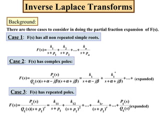
5. Inverse Laplace Transforms
Case 3: Repeated roots.
When we have repeated roots we find the coefficients of the
terms as follows:
[ ]|
111
)()( 1 psr
sFps
ds
d
k r
−=−
+=
[ ]|
121
)()(
!2 12
2
psr
sFps
ds
d
k r
−=−
+=
[ ]|
11
)()(
)!( 1 psj
sFps
dsjr
d
k r
jr
jr
−=+
−
= −
−

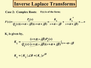
6. Inverse Laplace Transforms
Case 3: Repeated roots. Example
=
=
=
+
+
+
+=
+
+
=
2
1
1
2
211
2
)3()3()3(
)1(
)(
K
K
A
s
K
s
K
s
A
ss
s
sF
[ ] [ ] [ ][ ] )(____________________)( 33
tuteetf tt −−
++= ? ? ?

7. Inverse Laplace Transforms
Case 2: Complex Roots:
++
++
+
−+
=
++−+
= ...
)))()((
)(
)(
*
11
1
1
βαβαβαβα js
K
js
K
jsjssQ
sP
sF
F(s) is of the form;
K1 is given by,
θ
θ
βαβα
βα
βα
j
eKKK
jsjssQ
sPjs
K js
||||
))(()(
)()(
1
11
1
1
1
|
=∠=
++−+
−+
= −−=

8. Inverse Laplace Transforms
Case 2: Complex Roots:
βαβαβαβα
θθ
js
eK
js
eK
js
K
js
K
jj
++
+
−+
=
++
+
−+
−
11
*
11
|||





 −−−
+−=








++
+
−+
−
− tj
ete
j
e
tj
ete
j
eK
js
eK
js
eK
L
jj
βαββαθ
βαβα
θθ
1
||
|||| 111







 +
+
+
−=




 −−−
+−
2
)()(
|
1
|2
1
||
θβθβ
βαββαθ
tj
e
tj
eateK
tj
ete
j
e
tj
ete
j
eK

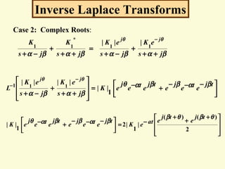
9. Inverse Laplace Transforms
[ ])cos(||2
|||
1
111
θβ
βαβα
α
θθ
+=








++
+
−+
−
−
−
teK
js
eK
js
eK
L t
jj
Case 2: Complex Roots:
Therefore:
You should put this in your memory:

10. Inverse Laplace Transforms
Complex Roots: An Example.
For the given F(s) find f(t)
o
jj
j
jss
s
K
ss
s
A
js
K
js
K
s
A
sF
jsjss
s
sss
s
sF
js
s
10832.0
)2)(2(
12
)2(
)1(
5
1
)54(
)1(
22
)(
)2)(2(
)1(
)54(
)1(
)(
|
|
2|1
0|
11
2
2
*
−∠=
+−
++−
=
++
+
=
=
++
+
=
++
+
−+
+=
++−+
+
=
++
+
=
+−=
=

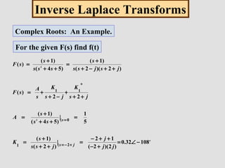
11. Inverse Laplace Transforms
Complex Roots: An Example. (continued)
We then have;
jsjss
sF
oo
++
+∠
+
−+
−∠
+=
2
10832.0
2
10832.02.0
)(
Recalling the form of the inverse for complex roots;
[ ] )(108cos(64.02.0)( 2
tutetf ot
−+= −

12. Inverse Laplace Transforms
Convolution Integral:
Consider that we have the following situation.
h(t)
x(t) y(t)
x(t) is the input to the system.
h(t) is the impulse response of the system.
y(t) is the output of the system.
System
We will look at how the above is related in the time domain
and in the Laplace transform.

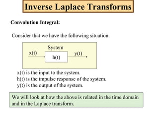
13. Inverse Laplace Transforms
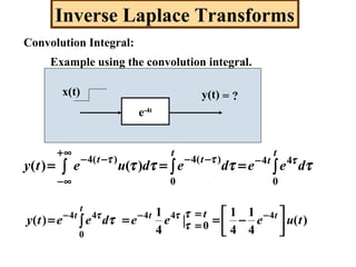
Convolution Integral:
In the time domain we can write the following:
∫∫
=
=
=
=
−=−=⊕=
tt
dxthdhtxthtxty
τ
τ
τ
τ
ττττττ
00
)()()()()()()(
In this case x(t) and h(t) are said to be convolved and the
integral on the right is called the convolution integral.
It can be shown that,
[ ] ( )sHsXsYthtxL )()()()( ==⊕
This is very important
* note

14. Inverse Laplace Transforms
Convolution Integral:
Through an example let us see how the convolution integral
and the Laplace transform are related.
We now think of the following situation:
x(t) y(t)
X(s) Y(s)
t
e 4−
h(t)
H(s)
)4(
1
+s

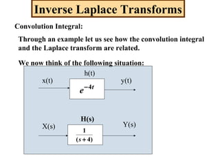
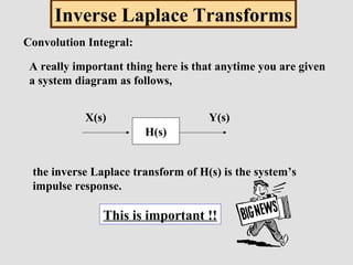
15. Inverse Laplace Transforms
Convolution Integral:
From the previous diagram we note the following:
[ ] [ ] [ ])()(;)()(;)()( thLsHtyLsYtxLsX ===
h(t) is called the system impulse response for the following
reason.
)()()( sHsXsY =
If the input x(t) is a unit impulse, δ(t), the L(x(t)) = X(s) = 1.
Since x(t) is an impulse, we say that y(t) is the impulse
response. From Eq A, if X(s) = 1, then Y(s) = H(s). Since,
Eq A
[ ] [ ]
.)(,
)()()()( 11
responseimpulsesystemthSo
thsHLresponseimpulsetysYL
=
==== −−

16. Inverse Laplace Transforms
Convolution Integral:
A really important thing here is that anytime you are given
a system diagram as follows,
H(s)
X(s) Y(s)
the inverse Laplace transform of H(s) is the system’s
impulse response.
This is important !!

17. Inverse Laplace Transforms
Convolution Integral:
Example using the convolution integral.
e-4t
x(t) y(t) = ?
∫∫∫
−−−
∞+
∞−
−−
===
t
t
t
tt
deededuety
0
44
0
)(4)(4
)()( ττττ τττ
)(
4
1
4
1
4
1
)( 444
0
44
| 0 tueeedeety tt
t
t t




−=== −−− =
=∫
τ
τ
ττ
τ

18. Inverse Laplace Transforms
Convolution Integral:
Same example but using Laplace.
x(t) = u(t)
s
sX
1
)( =
h(t) = e-4t
u(t)
4
1
)(
+
=
s
sH
[ ] )(1
4
1
)(
4
4141
4)4(
1
)(
4
tuety
sss
B
s
A
ss
sY
t−
−=
+
−=
+
+=
+
=

19. Inverse Laplace Transforms
Convolution Integral:
Practice problems:
?)(,
)2(
3
)(
2
)()( thiswhat
s
sYand
s
sXIfa
+
==
).(),()()()()( 6
thfindtutetyandtutxIfb t−
==
).(,
)4(
2
)()()()( 2
tyfind
s
sHandttutxIfc
+
==
Answers given on note page
[ ])(2)(5.1)( 2
tuetth t−
−= δ

20. Inverse Laplace Transforms
Circuit theory problem:
You are given the circuit shown below.
+_
• •
•
t = 0 6 k Ω
3 k Ω
1 0 0 µ F
+
_
v ( t )1 2 V
Use Laplace transforms to find v(t) for t > 0.

21. Circuit theory problem:
Inverse Laplace Transforms
We see from the circuit,
+_
• •
•
t = 0 6 k Ω
3 k Ω
1 0 0 µ F
+
_
v ( t )1 2 V
voltsxv 4
9
3
12)0( ==

22. Circuit theory problem:
Inverse Laplace Transforms
+
_
v c ( t ) i ( t )
3 k Ω
1 0 0 µ F
6 k Ω
( )
( ) 05
)(
0
)(
0)(
)(
=+
=+
=+
tv
dt
tdv
RC
tv
dt
tdv
tv
dt
tdv
RC
c
c
cc
c
c
Take the Laplace transform
of this equations including
the initial conditions on vc(t)

23. Circuit theory problem:
Inverse Laplace Transforms
)(4)(
5
4
)(
0)(54)(
0)(5
)(
5
tuetv
s
sV
sVssV
tv
dt
tdv
t
c
c
cc
c
c
−
=
+
=
=+−
=+

24. Stop