Downloaded 644 times
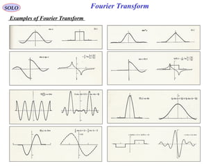
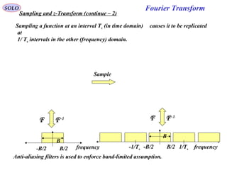
![Fourier Transform
( ) ( ){ } ( ) ( )∫
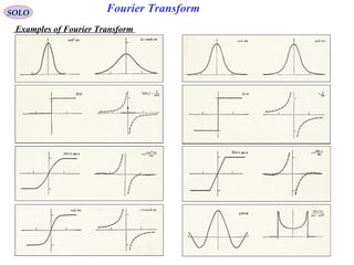
+∞
∞−
−== dttjtftfF ωω exp:F
SOLO
Jean Baptiste Joseph
Fourier
1768-1830
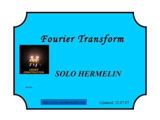
F (ω) is known as Fourier Integral or Fourier Transform
and is in general complex
( ) ( ) ( ) ( ) ( )[ ]ωφωωωω jAFjFF expImRe =+=
Using the identities
( ) ( )t
d
tj δ
π
ω
ω =∫
+∞
∞− 2
exp
we can find the Inverse Fourier Transform ( ) ( ){ }ωFtf -1
F=
( ) ( ) ( ) ( ) ( )
( ) ( )( ) ( ) ( ) ( ) ( )[ ]00
2
1
2
exp
2
expexp
2
exp
++−=−=−=
−=
∫∫ ∫
∫ ∫∫
∞+
∞−
∞+
∞−
∞+
∞−
+∞
∞−
+∞
∞−
+∞
∞−
tftfdtfd
d
tjf
d
tjdjf
d
tjF
ττδττ
π
ω
τωτ
π
ω
ωττωτ
π
ω
ωω
( ) ( ){ } ( ) ( )∫
+∞
∞−
==
π
ω
ωωω
2
exp:
d
tjFFtf -1
F
( ) ( ) ( ) ( )[ ]00
2
1
++−=−∫
+∞
∞−
tftfdtf ττδτ
If f (t) is continuous at t, i.e. f (t-0) = f (t+0)
This is true if (sufficient not necessary)
f (t) and f ’ (t) are piecewise continue in every finite interval1
2 and converge, i.e. f (t) is absolute integrable in (-∞,∞)( )∫
+∞
∞−
dttf](https://image.slidesharecdn.com/fouriertransform-140924230100-phpapp02/85/Fourier-transform-2-320.jpg)
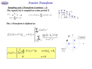
![Fourier TransformSOLO
( )tf
-1
F
F
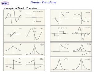
( )ωFProperties of Fourier Transform
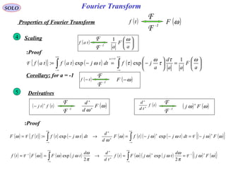
Linearity1
( ) ( ){ } ( ) ( )[ ] ( ) ( ) ( )ωαωαωαααα 221122112211 exp: FFdttjtftftftf +=−+=+ ∫
+∞
∞−
F
Symmetry2
( )tF
-1
F
F
( )ωπ −f2
( ) ( ) ( ) ( ) ( ) ( ) ( ) ( ) ( ) ( ){ }tFdttjtFf
dt
tjtFf
d
tjFtf
t
F=−=−⇒=⇒= ∫∫∫
+∞
∞−
+∞
∞−
↔
+∞
∞−
ωωπ
π
ωω
π
ω
ωω
ω
exp2
2
exp
2
exp
Proof:
Conjugate Functions3
( )tf *
-1
F
F
( )ω−*
F
Proof:
( ) ( ) ( ) ( ) ( ) ( ){ }tf
d
tjF
d
tjFtf ****
2
exp
2
exp 1-
F=−=−= ∫∫
+∞
∞−
→−
+∞
∞−
π
ω
ωω
π
ω
ωω
ωω](https://image.slidesharecdn.com/fouriertransform-140924230100-phpapp02/85/Fourier-transform-3-320.jpg)
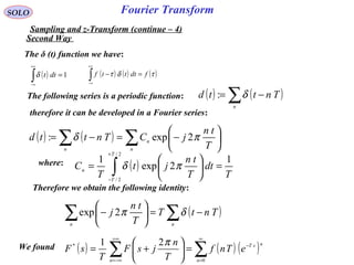
![Fourier TransformSOLO
( )tf
-1
F
F
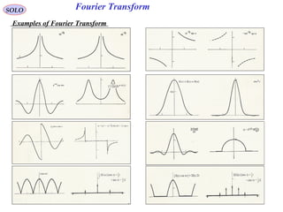
( )ωFProperties of Fourier Transform
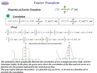
Modulation9
Shifting: for any a real8
Proof:
( ) ttf 0cos ω -1
F
F
( ) ( )[ ]00
2
1
ωωωω −++ FF
Proof:
( ) ( )[ ]tjtjt 000 expexp
2
1
cos ωωω −+=
( )atf −
-1
F
F ( ) ( )ωω ajF −exp ( ) ( )tajtf exp
-1
F
F ( )aF −ω
( ){ } ( ) ( ) ( ) ( )( ) ( ) ( )ωωττωτω
τ
Fajdajfdttjatfatf
at
−=+−=−−=− ∫∫
+∞
∞−
=−
+∞
∞−
expexpexp:F
( ) ( ){ } ( ) ( ) ( ) ( ) ( )( ) ( )aFdttajtfdttjtajtftajtf −=−−=−= ∫∫
+∞
∞−
+∞
∞−
ωωω expexpexp:expF
use shifting property with a=±ω0](https://image.slidesharecdn.com/fouriertransform-140924230100-phpapp02/85/Fourier-transform-8-320.jpg)
![( )atf −
-1
F
F ( ) ( )ωω ajF −exp
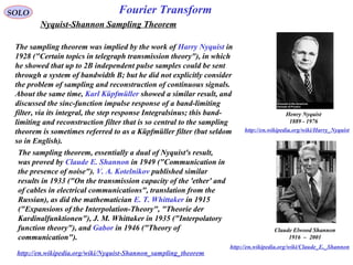
Fourier TransformSOLO
( )tf
-1
F
F
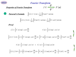
( )ωFProperties of Fourier Transform (Summary)
Linearity1
( ) ( ){ } ( ) ( )[ ] ( ) ( ) ( )ωαωαωαααα 221122112211 exp: FFdttjtftftftf +=−+=+ ∫
+∞
∞−
F
Symmetry2
( )tF
-1
F
F
( )ωπ −f2
Conjugate Functions3 ( )tf *
-1
F
F
( )ω−*
F
Scaling4 ( )taf
-1
F
F
a
F
a
ω1
Derivatives5 ( ) ( )tftj
n
−
-1
F
F ( )ω
ω
F
d
d
n
n
( )tf
td
d
n
n
-1
F
F
( ) ( )ωω Fj
n
Convolution6
( ) ( )tftf 21
-1
F
F ( ) ( )ωω 21
* FF( ) ( ) ( ) ( )∫
+∞
∞−
−= τττ dtfftftf 2121
:*
-1
F
F ( ) ( )ωω 21
FF
( ) ( ) ( ) ( )∫∫
+∞
∞−
+∞
∞−
= ωωω
π
dFFdttftf 2
*
12
*
1
2
1
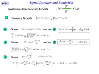
Parseval’s Formula7
Shifting: for any a real8
( ) ( )tajtf exp
-1
F
F ( )aF −ω
Modulation9 ( ) ttf 0
cos ω -1
F
F
( ) ( )[ ]00
2
1
ωωωω −++ FF
( ) ( ) ( ) ( ) ( ) ( )∫∫∫
+∞
∞−
+∞
∞−
+∞
∞−
−=−= ωωω
π
ωωω
π
dFFdFFdttftf 212121
2
1
2
1](https://image.slidesharecdn.com/fouriertransform-140924230100-phpapp02/85/Fourier-transform-9-320.jpg)
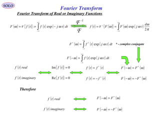
![Fourier Transform
SOLO
( ) realtf ( ) ( )ωω *
FF =−
( ) imaginarytf ( ) ( )ωω *
FF −=−
( ) realtf
( ) ( )
( ) ( )
−−=
−=
ωω
ωω
FF
FF
ImIm
ReRe
( ) imaginarytf
( ) ( )
( ) ( )
−=
−−=
ωω
ωω
FF
FF
ImIm
ReRe
( ) ( ) ( ) ( ){ } ( ) ( )∫
+∞
∞−
−==+= dttjtftfFjFF ωωωω exp:ImRe F
( ){ } ( ) ( ) ( ) ( ) ( )ωωω −==−−=− ∫∫
+∞
∞−
+∞
∞−
Fdttjtfdttjtftf expexpF
( ) ( ) ( )[ ] ( )tftftftf eveneven −=−+= 5.0: ( ) ( ) ( )[ ] ( )tftftftf oddodd −−=−−= 5.0:
( ) realtf
( ) ( ) ( )[ ] ( ){ } ( ) ( )[ ] ( )
( ) ( ) ( )[ ] ( ){ } ( ) ( )[ ] ( )
=−−=⇔−−=
=−+=⇔−+=
ωωω
ωωω
FjFFtftftftf
FFFtftftftf
evenodd
eveneven
Im5.05.0:
Re5.05.0:
F
F
( ) ( ) ( )[ ] ( ){ } ( ) ( )[ ] ( )
( ) ( ) ( )[ ] ( ){ } ( ) ( )[ ] ( )
=−−=⇔−−=
=−+=⇔−+=
ωωω
ωωω
FFFtftftftf
FjFFtftftftf
evenodd
eveneven
Re5.05.0:
Im5.05.0:
F
F
( ) imaginarytf
Fourier Transform of Real or Imaginary Functions (continue – 1)](https://image.slidesharecdn.com/fouriertransform-140924230100-phpapp02/85/Fourier-transform-11-320.jpg)
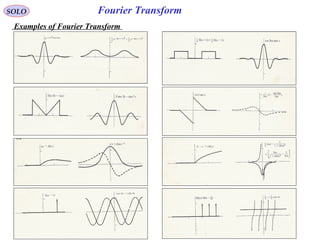
![Fourier Transform
ω
( )ωFRe
( )ωFIm
Real & Even
t
( )tfIm
( )tfRe
Real & Even
SOLO
ω
( )ωFRe
( )ωFIm
Imaginary & Odd
t
( )tfIm
( )tfRe
Real & Odd
ω
( )ωFRe
( )ωFIm
Imag. &Even
t
( )tfIm
( )tfRe
Imag.&
Even
ω
( )ωFRe
( )ωFIm
Real & Odd
t
( )tfIm
( )tfRe
Imag. & Odd
( ) realtf
( ) ( ) ( ) ( )[ ]tftftftf even −+== 5.0:
( ) ( ) ( ) ( )[ ]tftftftf even −+== 5.0:
( ) imaginarytf
( ){ } ( ){ } ( ) ( )[ ]
( ) ( )ωω
ωω
−==
−+==
FF
FFtftf even
ReRe
5.0FF
( ) ( )ωω *
FF =−
( ) ( ) ( ) ( )[ ]tftftftf odd
−−== 5.0:
( ){ } ( ){ } ( ) ( )[ ]
( ) ( )ωω
ωω
−−==
−−==
FjFj
FFtftf even
ImIm
5.0FF
( ) realtf ( ) ( )ωω *
FF =−
( ) ( )ωω *
FF −=−
( ) ( ) ( ) ( )[ ]tftftftf odd −−== 5.0:
( ){ } ( ){ } ( ) ( )[ ]
( ) ( )ωω
ωω
−==
−+==
FjFj
FFtftf even
ImIm
5.0FF
( ) imaginarytf ( ) ( )ωω *
FF −=−
( ){ } ( ){ } ( ) ( )[ ]
( ) ( )ωω
ωω
−−==
−−==
FF
FFtftf even
ReRe
5.0FF
Fourier Transform of Real or Imaginary Functions (continue – 2)](https://image.slidesharecdn.com/fouriertransform-140924230100-phpapp02/85/Fourier-transform-12-320.jpg)
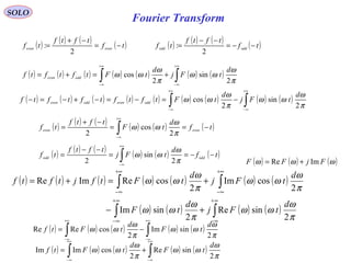
![Fourier Transform
SOLO
( ) ( ){ } ( ) ( ) ( ) ( )[ ] ( ) ( )[ ]
( ) ( )[ ] ( ) ( ) ( )[ ] ( )∫∫
∫∫
∞+
∞−
∞+
∞−
+∞
∞−
+∞
∞−
+−+=
−+=−==
dtttftfjdtttftf
dttjttftfdttjtftfF
oddevenoddeven
oddeven
ωω
ωωωω
sincos
sincosexp:F
( ) ( ) ( )[ ] ( )tftftftf eveneven
−=−+= 5.0: ( ) ( ) ( )[ ] ( )tftftftf oddodd
−−=−−= 5.0: ( ) ( ) ( )tftftf oddeven
+=
( ) ( ) ( ) ( ) ( ) ( ) ( )
( )
( ) ( ) ( ) ( ) ( )∫∫∫∫∫∫
+∞+∞+∞+∞
−→
∞−
+∞
∞−
=+−=+=
0000
0
cos2coscoscoscoscos dtttfdtttfdfdtttfdtttfdtttf eveneven
f
eveneven
t
eveneven
even
ωωττωτωωω
τ
τ
( ) ( ) ( ) ( ) ( ) ( ) ( )
( )
( ) ( ) ( ) 0coscoscoscoscos
000
0
=+−=+= ∫∫∫∫∫
+∞+∞
−
+∞
−→
∞−
+∞
∞−
dtttfdfdtttfdtttfdtttf odd
f
oddodd
t
oddodd
odd
ωττωτωωω
τ
τ
( ) ( ) ( ) ( ) ( ) ( ) ( )
( )
( ) ( ) ( ) 0sinsinsinsinsin
000
0
=+−−=+= ∫∫∫∫∫
+∞+∞+∞
−→
∞−
+∞
∞−
dtttfdfdtttfdtttfdtttf even
f
eveneven
t
eveneven
even
ωττωτωωω
τ
τ
( ) ( ) ( ) ( ) ( ) ( ) ( )
( )
( ) ( ) ( ) ( ) ( )∫∫∫∫∫∫
+∞+∞+∞
−
+∞
−→
∞−
+∞
∞−
=+−−=+=
0000
0
sin2sinsinsinsinsin dtttfdtttfdfdtttfdtttfdtttf oddodd
f
oddodd
t
oddodd
odd
ωωττωτωωω
τ
τ
Therefore ( ) ( ){ } ( ) ( ) ( ) ( ) ( ) ( )∫∫∫
+∞+∞+∞
∞−
−=−==
00
sin2cos2exp: dtttfjdtttfdttjtftfF oddeven ωωωω F
( ) ( ) ( )[ ] ( ) ( )∫
+∞
=−+=
0
cos25.0 dtttfFFF eveneven ωωωω ( ) ( ) ( )[ ] ( ) ( )∫
+∞
=−−=
0
sin25.0 dtttfjFFF oddodd ωωωω
Odd and Even Parts](https://image.slidesharecdn.com/fouriertransform-140924230100-phpapp02/85/Fourier-transform-13-320.jpg)
![Fourier Transform
( ) ( ){ } ( ) ( ) ( ) ( )[ ] ( ) ( )[ ]
( ) ( ) ( ) ( )[ ] ( ) ( ) ( ) ( )[ ]∫∫
∫∫
∞+
∞−
∞+
∞−
+∞
∞−
+∞
∞−
++−=
++===
π
ω
ωωωω
π
ω
ωωωω
π
ω
ωωωω
π
ω
ωωω
2
cosImsinRe
2
sinImcosRe
2
sincosImRe
2
exp:
d
tFtFj
d
tFtF
d
tjtFjF
d
tjFFtf -1
F
SOLO
( ) 00: <∀= ttfCausal
Causal Functions
A causal functions is a equal zero for negative t
( ) ( ) ( )[ ] ( )tftftftf eveneven
−=−+= 5.0: ( ) ( ) ( )[ ] ( )tftftftf oddodd
−−=−−= 5.0:
Since
and ( ) 0>− ttf we have ( ) ( ) ( ) 022 >== ttftftf oddeven
( ) realtf
( ) ( ){ } ( ) ( ) ( ) ( )[ ]∫
+∞
∞−
−==
π
ω
ωωωωω
2
sinImcosRe
d
tFtFFtf -1
F
( ) causalrealtf & ( ) ( ) ( ) ( ) ( ) ( ) ( )
( ) ( ) ( ) ( ) 0
2
sinIm4
2
cosRe4
2
sinIm22
2
cosRe22
00
>−==
−====
∫∫
∫∫
∞+∞+
+∞
∞−
+∞
∞−
t
d
tF
d
tF
d
tFtf
d
tFtftf oddeven
π
ω
ωω
π
ω
ωω
π
ω
ωω
π
ω
ωω
( ) ( )
( ) ( )
−−=
−=
ωω
ωω
FF
FF
ImIm
ReRe
( ) ( ) ( ) ( ) ( ) 0sinIm
2
cosRe
2
00
>−== ∫∫
+∞+∞
tdtFdtFtf ωωω
π
ωωω
π](https://image.slidesharecdn.com/fouriertransform-140924230100-phpapp02/85/Fourier-transform-14-320.jpg)
![Fourier TransformSOLO
( ) 00: <∀= ttfCausalReal & Causal Functions ( ) ( ) ( ) 022 >== ttftftf oddeven
( ) causalrealtf & ( ) ( ) ( ) ( ) ( ) 0sinIm
2
cosRe
2
00
>−== ∫∫
+∞+∞
tdtFdtFtf ωωω
π
ωωω
π
( ) ( ) ( ) ( ) ( ) ( )[ ]∫
+∞
∞−
−=+= dttjttfFjFF ωωωωω sincosImRe
( ) ( ) ( ) ( ) ( ) ( ) ( ) ( ) ( )∫ ∫∫ ∫∫
+∞
∞−
+∞+∞
∞−
+∞+∞
∞−
−=
−== dtduttuuFdttdutuuFdtttfF ω
π
ω
π
ωω cossinIm
2
cossinIm
2
cosRe
00
( ) ( ) ( ) ( ) ( ) ( ) ( ) ( ) ( )∫ ∫∫ ∫∫
+∞
∞−
+∞+∞
∞−
+∞+∞
∞−
−=
−=−= dvdtttvvFdttdvtvvFdtttfF ω
π
ω
π
ωω sincosRe
2
sincosRe
2
sinIm
00
Therefore
( ) ( ) ( ) ( )∫ ∫
+∞
∞−
+∞
−= dtduttuuFF ω
π
ω cossinIm
2
Re
0
( ) ( ) ( ) ( )∫ ∫
+∞
∞−
+∞
−= dtdvttvvFF ω
π
ω sincosRe
2
Im
0
But also
( ) ( ) ( ) ( )∫ ∫
+∞
∞−
+∞
= dtduttuuFF ω
π
ω coscosRe
2
Re
0
( ) ( ) ( ) ( )∫ ∫
+∞
∞−
+∞
= dtdvttvvFF ω
π
ω sinsinRe
2
Im
0
Real & Causal Functions
Real & Causal Functions
( ) ( )
( ) ( )
−−=
−=
ωω
ωω
FF
FF
ImIm
ReRe](https://image.slidesharecdn.com/fouriertransform-140924230100-phpapp02/85/Fourier-transform-15-320.jpg)
![Fourier Transform
( )
>
<
=Π
2
1
0
2
1
1
t
t
t
2
1
2
1
−
( )tΠ
t
Rectangle
1
( ) ( )
−<−
<
>
=
τ
ττ
τ
τ
t
tt
t
t
2/1
2/
2/1
lim
Limiter τ
( )[ ] ( )tt sgnlimlim2 0
=→ ττ
0
( )tτlim
t
2/1
2/1−
τ
τ−
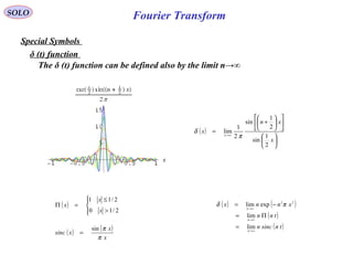
SOLO
Special Symbols
( )
>
<−
=Λ
10
11
t
tt
t
11−
( )tΛ
t
Triangle
1
( )
<
>
=
00
01
t
t
tH
0
( )tH
t
Heaviside
unit step
1
( )
<−
>
=
01
01
sgn
t
t
t
0
( )tsgn
t
Signum 1
1−
0
( )t
td
d
τlim
t
( )τ2/1
ττ−
Area = 1td
d](https://image.slidesharecdn.com/fouriertransform-140924230100-phpapp02/85/Fourier-transform-23-320.jpg)
![Fourier Transform
( ) ( ) ( )
( )
≠
=∞
=
>
≤
=
<−
≤
>
=
= →→→
00
0
0
2/1
lim
2/1
2/
2/1
limlimlim: 000
t
t
t
t
t
tt
t
td
d
t
td
d
t
τ
ττ
τ
ττ
τ
δ ττττ
SOLO
Special Symbols
0
( )t
td
d
τlim
t
( )τ2/1
ττ−
Area = 1td
d
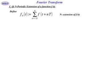
δ (t) function
Since ( )( ) ( )tt sgn
2
1
limlim
0
=
→
ττ
we have also
δ (t) function is defined as:
( ) ( )t
td
d
t sgn
2
1
=δ
0
( )t
td
d
τlim
t
( )τ2/1
ττ−
Area = 1
0 t
( )tδ
Area = 1
0→τ
( ) ( )
−<−
<
>
=
τ
ττ
τ
τ
t
tt
t
t
2/1
2/
2/1
lim
Limiter τ
( )[ ] ( )tt sgnlimlim2
0
=
→ ττ
0
( )tτlim
t
2/1
2/1−
τ
τ−](https://image.slidesharecdn.com/fouriertransform-140924230100-phpapp02/85/Fourier-transform-24-320.jpg)
![Fourier TransformSOLO
Special Symbols
Properties of δ (t) function
0
( )t
td
d
τlim
t
( )τ2/1
ττ−
Area = 1
0 t
( )tδ
Area = 1
0→τ
( ) ( )tt −= δδδ (t) is a even function:2
( )
( )
≠
=∞
=
>
≤
=
→
00
0
0
2/1
lim
0
t
t
t
t
t
τ
ττ
δ τ
1
3 ( ) ( )
( ) ( )
( ) ( ) ( ) ( )[ ]00
2
1
++−=−=− ∫∫
+∞
∞−
−=+∞
∞−
τττδτδ
δδ
ffdtttfdtttf
uu
Proof:
( ) ( )
( ) ( )
( ) ( ) ( ) ( )[ ] ( ) ( )
( ) ( ) ( ) ( ) ( ) ( ) ( ) ( ) ( ) ( )[ ]
( ) ( )[ ]00
2
1
00
2
1
lim
2
1
lim
sgn
2
1
limsgn
2
1
limsgnlim
2
1
lim
0
0
sgn
2
1
++−=
++−−−−+−+=
−+−+=
−−−=−=−
→∞
+
−
−
→∞
+
−
→∞
+
−→∞
+
−
→∞
=+
−
→∞
∫∫
∫∫∫
ττ
ττ
ττττδ
τ
τ
δ
ff
fTfTffTfTftfdtfdTfTf
tfdtttftdtfdtttf
T
T
T
T
T
T
T
T
TT
T
T
T
t
dt
d
tT
T
T
4 Fourier Transform ( ){ } ( ) ( ) ( ) ( ) 10exp
2
1
0exp
2
1
exp =++−=−= ∫
+∞
∞−
jjdttjtt ωδδF](https://image.slidesharecdn.com/fouriertransform-140924230100-phpapp02/85/Fourier-transform-25-320.jpg)
![Fourier Transform
( )
−=
+
=
=
=
−=
=
+
=
→
→
→
→
→
−
→
→
εεε
εε
εε
επ
εεπ
ε
ε
ε
π
δ
ε
ε
ε
ε
ε
ε
ε
ε
ε
x
Ln
x
x
J
x
Ai
x
x
x
x
x
x
2
exp
1
lim
11
lim
1
lim
sin
1
lim
4
exp
2
1
lim
lim
lim
1
2
0
/1
0
0
0
2
0
1
0
220
SOLO
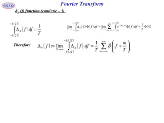
Special Symbols
δ (t) function
The δ (t) function can be defined as the following limit as ε→0
Ai is the Airry function,
( ) ∫
∞
+=
0
3
3
cos
1
dttx
t
xAi
π ( ) ( )[ ]∫
+
−
−−=
π
π
τττ
π
dxnjxJn
sinexp
2
1
Friedrich Wilhelm
Bessel
1784 - 1846
Edmond Nicolas
Laguerre
1834 - 1886
Jn (x) is the Bessel function of the first kind,
and Ln (x) is the Laguerre polynomial of arbitrary positive order.](https://image.slidesharecdn.com/fouriertransform-140924230100-phpapp02/85/Fourier-transform-26-320.jpg)
![Fourier TransformSOLO
δ (t) function
( )
>
≤
=
2
0
2
1
:
02
τ
τ
τδ
π
τ
t
te
t
tfj
Use
It’s Fourier Transform is
( ) ( ) ( )
( )
( )
( )[ ]
( )τπ
τπ
πττ
δ
τ
τ
πτ
τ
ππ
ττ
ff
ff
ffj
e
dtedtetf
tffj
tffjtfj
−
−
=
−
===∆
+
−
−+
−
−
∞+
∞−
−
∫∫ 0
0
2/
2/0
22/
2/
22 sin
2
11 0
0
For any function φ (t), defined at t=0- and t=0+, we have
( ) ( ) ( ) ( ) ( )
( ) ( ) ( ) ( )[ ]+−
−
→
+
→
−
→
+
→
+
−
→
+∞
∞−
→
+=+=
+==
−
+
−
+
∫∫∫∫
00
2
11
lim
1
lim
1
lim
1
lim
1
limlim
0
2/
0
2/
0
0
0
2/
2
0
2/
0
2
0
2/
2/
2
00
000
ϕϕϕ
τ
ϕ
τ
ϕ
τ
ϕ
τ
ϕ
τ
ϕδ
τ
τ
τ
τ
τ
π
τ
τ
π
τ
τ
τ
π
τ
τ
τ
tttt
dttedttedttedttt tfjtfjtfj
( ) ( )tt δδτ
τ
=
→0
lim](https://image.slidesharecdn.com/fouriertransform-140924230100-phpapp02/85/Fourier-transform-28-320.jpg)
![Fourier Transform
( )
>
≤
=
2
0
2
1
:
02
τ
τ
τδ
π
τ
t
te
t
tfj
SOLO
δ (t) function
( ) ( )[ ]
( )τπ
τπ
τ
ff
ff
f
−
−
=∆
0
0sin
( ) ( )tt δδτ
τ
=
→0
lim ( ) ( )[ ]
( )
1
sin
limlim
0
0
00
=
−
−
=∆
→→ τπ
τπ
τ
τ
τ ff
ff
f
( )[ ]
( )τπ
τπ
ff
ff
−
−
0
0sin
( ) ∫
+∞
∞−
= fdet tfj π
δ 2](https://image.slidesharecdn.com/fouriertransform-140924230100-phpapp02/85/Fourier-transform-29-320.jpg)
![Fourier Transform
( )
∆>−
∆≤−
∆=∆
2/0
2/
1
:
0
0
fff
fff
ffS f
SOLO
δ (f) function
Define:
In the time domain we obtain:
( ) ( ) ( )
( )
tfj
ff
ff
tfjff
ff
tfjtfj
ff e
tf
tf
tj
e
f
fde
f
fdefSts 0
0
0
0
0
2
2/
2/
22/
2/
22 sin
2
11 π
π
ππ
π
π
π ∆
∆
=
∆
=
∆
==
∆+
∆−
∆+
∆−
+∞
∞−
∆∆ ∫∫
For any function Φ (f), defined at f=f0- and f=f 0+ , we have
( ) ( ) ( ) ( ) ( )
( ) ( ) ( ) ( )[ ]+−
−
+
+
−
Φ+Φ=Φ
∆
+Φ
∆
=
Φ
∆
+Φ
∆
=Φ
∆
=Φ
∆−
→∆
∆+
→∆
∆−
→∆
∆+
→∆
∆+
∆−
→∆
+∞
∞−
∆
→∆ ∫∫∫∫
00
2/
0
2/
0
2/
0
2/
0
2/
2/
00
2
11
lim
1
lim
1
lim
1
lim
1
limlim
0
0
0
0
0
0
0
0
0
0
ffff
f
ff
f
dff
f
dff
f
dff
f
dfffS
f
ff
f
ff
f
f
f
ff
f
ff
f
f
ff
ff
f
f
f
( ) ( )0
0
lim fffS f
f
−=∆
→∆
δ
( ) ( )0
0
:lim fffS f
f
−=∆
→∆
δ ( ) tfj
f
f
ets 02
0
lim π
=∆
→∆
( ) ( )
∫
+∞
∞−
−−
=− tdeff tffj 02
0
π
δ](https://image.slidesharecdn.com/fouriertransform-140924230100-phpapp02/85/Fourier-transform-30-320.jpg)
![Fourier Transform
( ) ( )∑−=
+=
N
Nn
N Tntt δδ :
SOLO
δN (f) function
Define
Let find the Fourier transform of δN (f)
( ) ( ) ( )
( )[ ]
[ ]
( )Tf
TNf
ee
j
j
ee
eee
eee
e
ee
etdenTttdetf
TfjTfj
TNfjTNfj
TfjTfjTfj
TNfjTNfj
Tfj
Tfj
NTfjTNfj
N
Nn
Tnfj
N
Nn
tfjtfj
NN
π
π
δδ
ππ
ππ
πππ
ππ
π
π
ππ
πππ
sin
2
1
2sin
2
2
1
1
2
1
2
2
1
2
2
1
2
2
1
2
2
1222
222
+
=
−
−
=
=
−
−
=
−
−
=
=+==∆
−
+−
+
−
+
+−
+−
−=−=
+∞
∞−
−
+∞
∞−
−
∑∑ ∫∫
We can see that
( ) ( )[ ]
( )
( )[ ]
( )
( ) ,2,1,0
sin
12sin
sin
1212sin
±±=∆=
+
=
+
+++
=
+∆ kf
Tf
TNf
kTf
NkTNf
T
k
f NN
π
π
ππ
ππ
N-extension of δ (t)](https://image.slidesharecdn.com/fouriertransform-140924230100-phpapp02/85/Fourier-transform-32-320.jpg)
![Fourier TransformSOLO
δN (f) function (continue – 1)
( ) ( )∑−=
+=
N
Nn
N Tntt δδ : ( ) ( )[ ]
( ) ∑−=
=
+
=∆
N
Nn
Tnfj
N e
Tf
TNf
f π
π
π 2
sin
12sin
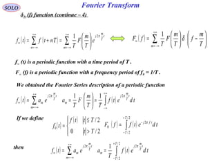
δN (t) is a periodic function with a time period of T .
ΔN (f) is a periodic function with a frequency period of f0 = 1/T .
( )
( )
( )
( )
( )
( )
( )
[ ]
Tn
n
TTnj
e
dfedff
N
Nn
n
n
N
Nn
T
T
TnfjN
Nn
T
T
Tnfj
T
T
N
1sin1
2
00
01
2/1
2/1
22/1
2/1
2
2/1
2/1
====∆ ∑∑∑ ∫∫ −=
≠←
=←
−=
−
−−=
+
−
+
−
π
π
π
π
π](https://image.slidesharecdn.com/fouriertransform-140924230100-phpapp02/85/Fourier-transform-33-320.jpg)
![Fourier TransformSOLO
δN (f) function (continue – 2)
When N → ∞ the peak goes to infinity and the null-to-null bandwidth goes to zero.
This resembles to a delta function. To prove that this is the case let compute:
ΔN (f) is a periodic function with a frequency period of f0 = 1/T , with peak amplitude of
(2 N+1) and null-to-null bandwidth of 2/ [(2N+1) T].
( )
( )
( )
T
dff
T
T
N
1
2/1
2/1
=∆∫
+
−
( ) ( )
( )
( )
( )
( )
( )
( )0
1
limlim
2/1
2/1
2
2/1
2/1
Φ=Φ=Φ∆ ∑ ∫∫ −=
+
−
∞→
+
−
∞→ T
dffedfff
N
Nn
T
T
Tnfj
N
T
T
N
N
π](https://image.slidesharecdn.com/fouriertransform-140924230100-phpapp02/85/Fourier-transform-34-320.jpg)
![Fourier TransformSOLO
δN (f) function (continue – 4)
Let compute the convolution between f (t) and δN (f)
( ) ( ) ( ) ( ) ( ) ( ) ( ) ( )tfTntfdTntfdTntfttf N
N
Nn
N
Nn
N
Nn
N =+=+−=+−=∗ ∑∑ ∫∫ ∑ −=−=
+∞
∞−
+∞
∞− −=
ττδτττδτδ :
Therefore ( ) ( ) ( )ttftf NN δ∗=
Using this relation the Fourier Transform of fN (t) is given by
( ) ( ) ( ) ( ) ( )[ ]
( )Tf
TfN
fFffFfF NN
π
π
sin
12sin +
=∆= ( ) ( ) ( ) ( )Tntfttftf
N
Nn
NN +=∗= ∑−=
δ
If N → ∞ then
( ) ( ) ( ) ( )
( ) ∑∑
∑
∞+
−∞=
∞+
−∞=
+∞
−∞=
∞∞
−
=
−=
−=∆=
mm
m
T
m
f
T
m
F
TT
m
ffF
T
T
m
f
T
fFffFfF
δδ
δ
11
1
( ) ( )
∑
∑
∑
∞+
−∞=
∞+
−∞=
−
+∞
−∞=
∞
=
−
=
+=
m
t
T
m
j
m
n
e
T
m
F
T
T
m
f
T
m
F
T
Tntftf
π
δ
2
1
1
1
F](https://image.slidesharecdn.com/fouriertransform-140924230100-phpapp02/85/Fourier-transform-36-320.jpg)
![Fourier Transform
( ) ( ){ } ( ) ( )∫
+∞
∞−
−== dttjtftfF νπνπ 2exp:2 F
( ) ( ) ( )∑∑
∞
=
−
+∞
−∞=
=
+=
0
* 21
n
nsT
n
eTnf
T
n
jsF
T
sF
π
( ) ( ){ } ( ) ( )∫
+∞
∞−
== ννπνπνπ dtjFFtf 2exp2:2-1
F
SOLO
Sampling and z-Transform (continue – 5)
We found
Using the definition of the Fourier Transform and it’s inverse:
we obtain ( ) ( ) ( )∫
+∞
∞−
= ννπνπ dTnjFTnf 2exp2
( ) ( ) ( ) ( ) ( ) ( )∑∫∑
∞
=
+∞
∞−
∞
=
−=−=
0
111
0
*
exp2exp2exp
nn
n
sTndTnjFsTTnfsF ννπνπ
( ) ( ) ( )[ ]∫ ∑
+∞
∞−
+∞
−∞=
−−== 111
*
2exp22 νννπνπνπ dTnjFjsF
n
( ) ( ) ∑∫ ∑
+∞
−∞=
+∞
∞−
+∞
−∞=
−=
−−==
nn T
n
F
T
d
T
n
T
FjsF νπνννδνπνπ 2
11
22 111
*
We recovered (with –n instead of n) ( ) ∑
+∞
−∞=
+=
n T
n
jsF
T
sF
π21*
Second Way (continue)
Making use of the identity: with 1/T instead of T
and ν - ν 1 instead of t we obtain: ( )[ ] ∑∑
−−=−−
nn T
n
T
Tnj 11
1
2exp ννδννπ
( )∑∑ −=
−
nn
TntT
T
tn
j δπ2exp](https://image.slidesharecdn.com/fouriertransform-140924230100-phpapp02/85/Fourier-transform-56-320.jpg)
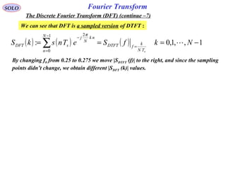
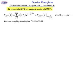
![Fourier TransformSOLO
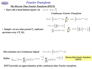
The Discrete Time Fourier Transform (DTFT) (continue-1)
• Signal can be recovered if Fourier spectrum of the sampling signal do not overlap.
Discretization of a Continuous Signal ( ) ( )∫
+∞
∞−
== fdefSTnts sTnfj
s
π2
DTFT-1
DTF
T
Discrete Time Fourier Transform
(DTFT)
( ) ( ) ( )∑∑
∞+
−∞=
−
=
∞+
−∞=
−
==
n
n
f
f
j
s
T
f
n
Tnfj
sDTFT
s
s
s
s
eTnseTnsfS
π
π
2
1
2
:
We can see that
( ) ( ) ( ) ( )∑∑
∞+
−∞=
−
−∞+
−∞=
+
−
===+
n
DTFT
nkj
n
f
f
j
s
n
n
f
fkf
j
ssDTFT fSeeTnseTnsfkfS ss
s
1
2
22
π
ππ
The Discrete Time Fourier Transform SDTFT (fs) is periodic with period fs.
Let compute
( ) ( )
( )
( )
( )
( )
( )
( ) ( ) ( )[ ]
( )
( )∑ ∑
∑ ∫∫ ∑∫
∞+
−∞=
∞+
−∞=
=←
≠←
+
−
−
∞+
−∞=
+
−
−
+
−
∞+
−∞=
−
+
−
=
−
−
=
−
=
==
n
s
sn
nm
nm
ss
f
fs
nm
f
f
j
s
n
f
f
nm
f
f
j
s
f
f n
nm
f
f
j
s
f
f
m
f
f
j
DTFT
Tms
Tnm
nm
fTns
f
nm
j
e
Tns
fdeTnsdfeTnsdfefS
s
s
s
s
s
s
s
s
s
s
s
s
1sin
2
1
0
2/
2/
2
2/
2/
22/
2/
22/
2/
2
π
π
π
π
πππ
( ) ( )∑
+∞
−∞=
−
=
n
Tnfj
sDTFT
s
eTnsfS π2
: ( ) ( )
( )
( )
∫
+
−
=
s
s
s
T
T
nTfj
DTFTss dfefSTTns
2/1
2/1
2π](https://image.slidesharecdn.com/fouriertransform-140924230100-phpapp02/85/Fourier-transform-61-320.jpg)
![Fourier TransformSOLO
The Discrete Time Fourier Transform (DTFT) (continue-2)
Normalization of the frequency
DTFT-1
DTFT
( ) ( )∑
+∞
−∞=
−
=
n
Tnfj
sDTFT
s
eTnsfS π2
: ( ) ( )
( )
( )
∫
+
−
=
s
s
s
T
T
nTfj
DTFTss dfefSTTns
2/1
2/1
2π
( ) ( )[ ]
[ ]2/1,2/1
2/1,2/1
:
*
*
+−∈
+−∈
=
f
TTf
Tff
ss
s
( ) ( )∑
+∞
−∞=
−
=
n
nfj
DTFT ensfS *2*
: π
DTFT-1
DTFT
( ) ( )∫
+
−
=
2/1
2/1
*2
** dfefSns nfj
DTFT
π
Example ( ) 1,,1,002
−== −
NneAns nfj
π
( ) ( )
( )
( )
( ) ( )
( ) ( )
( )
( )
( )[ ]
( )[ ]
( )( )1*
0
0
*
*
**
**
*2
*21
0
*2*
0
0
0
00
00
0
0
0
*sin
*sin
1
1
−−−
−−
−−
−−−
−−−
−−
−−−
=
−−
−
−
=
−
−
=
−
−
== ∑
Nffj
ffj
Nffj
ffjffj
NffjNffj
ffj
NffjN
n
nffj
DTFT
e
ff
Nff
A
e
e
ee
ee
A
e
e
AeAfS
π
π
π
ππ
ππ
π
π
π
π
π
|SDTFT(f*)|
Normalized Frequency](https://image.slidesharecdn.com/fouriertransform-140924230100-phpapp02/85/Fourier-transform-62-320.jpg)
![Fourier Transform
( ) ( )∑
−
=
−
=
1
0
2
:
N
n
nk
N
j
sDFT eTnskS
π
SOLO
The Discrete Fourier Transform (DFT)
Assume a periodic sequence, sampled at a time period Ts, such that s (n Ts) = s [(n+kN) Ts]
The Discrete Fourier Transform (DFT) requires an input function that is discrete
and whose non-zero values have a limited (finite) duration.
Unlike the Discrete-time Fourier transform (DTFT), it only evaluates enough frequency
components to reconstruct the finite segment that was analyzed. Its inverse transform
cannot reproduce the entire time domain, unless the input happens to be periodic (forever).
Therefore it is often said that the DFT is a transform for Fourier analysis of finite-domain
discrete-time functions
For the sequence s (0), s (Ts),…,s [(N-1) Ts] we define the Discrete Fourier Transform:](https://image.slidesharecdn.com/fouriertransform-140924230100-phpapp02/85/Fourier-transform-64-320.jpg)
![Fourier Transform
( ) ( ) ( )∑∑
−
=
−
=
−
==
1
0
1
0
2
:
N
n
nk
s
N
n
nk
N
j
sDFT WTnseTnskS
π
SOLO
The Discrete Fourier Transform (DFT) (continue – 1)
For the sequence s (0), s (Ts),…,s [(N-1) Ts] we define the Discrete Fourier Transform:
where is a primitive N'th root of unity
and is periodic
N
j
eW
π2
:
−
=
n
Nm
N
j
n
N
j
Nmn
N
j
Nmn
WeeeW =
=
=
−−
+
−
+
1
222 πππ
( )
( )
( )
( )
( )
( ) ( ) ( ) ( ) ( )
( ) ( ) ( ) ( ) ( )
( ) ( ) ( ) ( ) ( )
( ) ( ) ( ) ( ) ( )
( ) ( ) ( ) ( ) ( )
[ ]
( )
( )
( )
( )[ ]
( )[ ]
N
N
N s
s
s
s
s
s
W
NNNNNNN
NNNNNNN
NN
NN
NN
S
DFT
DFT
DFT
DFT
DFT
TNs
TNs
Ts
Ts
Ts
WWWWW
WWWWW
WWWWW
WWWWW
WWWWW
NS
NS
S
S
S
⋅−
⋅−
⋅
⋅
⋅
=
−
−
−−−−−−−
−−−−−−−
−−
−−
−−
1
2
2
1
0
1
2
2
1
0
1121211101
1222221202
1222221202
1121211101
1020201000
[ ] NNN sWS = [ ]NW is a Vandermonde type of Matrix](https://image.slidesharecdn.com/fouriertransform-140924230100-phpapp02/85/Fourier-transform-65-320.jpg)
![Fourier TransformSOLO
The Discrete Fourier Transform (DFT) (continue – 2)
nNmn
WW =+
[ ] [ ] N
H
NN I
N
WW
1
=
N
j
eW
π2
−
= 1
2
* −
== WeW N
j
π
[ ]
( ) ( ) ( ) ( ) ( )
( ) ( ) ( ) ( ) ( )
( ) ( ) ( ) ( ) ( )
( ) ( ) ( ) ( ) ( )
( ) ( ) ( ) ( ) ( )
=
−−−−−−−
−−−−−−−
−−
−−
−−
1121211101
1222221202
1222221202
1121211101
1020201000
NNNNNNN
NNNNNNN
NN
NN
NN
N
WWWWW
WWWWW
WWWWW
WWWWW
WWWWW
W
[ ] [ ]
( ) ( ) ( ) ( ) ( )
( ) ( ) ( ) ( ) ( )
( ) ( ) ( ) ( ) ( )
( ) ( ) ( ) ( ) ( )
( ) ( ) ( ) ( ) ( )
==
−+−−+−−−−−−
−+−−+−−−−−−
+−+−−−
+−+−−−
+−+−−−
1112121110
2122222120
2122222120
1112121110
0102020100
*
NNNNNNN
NNNNNNN
NN
NN
NN
T
N
H
N
WWWWW
WWWWW
WWWWW
WWWWW
WWWWW
WW
Let multiply those two matrices
[ ] [ ]( )( ) ( ) ( ) ( ) ( ) ( ) ( ) ( ) ( )
( )
( )
( )
( )
( )
( )
=
≠=
−
−
=
−
−
==
+++++=
−
−
−
−−
=
−
+−−−−
∑
mkN
mk
W
W
W
W
W
WWWWWWWWWW
mk
mk
N
mk
NmkN
j
jmk
mNNkmjjkmkmk
mk
H
NN
0
1
1
1
1
1
1
0
111100
,
Where IN is the NxN identity matrix](https://image.slidesharecdn.com/fouriertransform-140924230100-phpapp02/85/Fourier-transform-66-320.jpg)
![Fourier Transform
( ) ( ) ( )∑∑
−
=
−
=
−
==
1
0
1
0
2
:
N
n
nk
s
N
n
nk
N
j
sDFT WTnseTnskS
π
SOLO
The Discrete Fourier Transform (DFT) (continue – 3)
For the sequence s (0), s (Ts),…,s [(N-1) Ts] we defined the Discrete Fourier Transform:
[ ] NNN sWS = [ ]NW is a Vandermonde type of Matrix
We found that
[ ] [ ] N
H
NN I
N
WW
1
= Where IN is the NxN identity matrix
Therefore the Inverse Discrete Fourier Transform (IDFT) is
[ ] N
H
NN SW
N
s
1
=
( ) ( ) ( )∑∑
−
=
−
=
−
==
1
0
21
0
11 N
n
nk
N
j
DFT
N
k
nk
DFTs ekS
N
WkS
N
Tns
π
D.F.T.
I.D.F.T.](https://image.slidesharecdn.com/fouriertransform-140924230100-phpapp02/85/Fourier-transform-67-320.jpg)
![Fourier TransformSOLO
The Discrete Fourier Transform (DFT) (continue – 4)
Second way to find the Inverse Discrete Fourier Transform (IDFT). Let compute:
( ) ( )
( )
( )
( )
∑ ∑∑∑∑
−
=
−
=
−−−
=
−
=
−−−
=
+
==
1
0
1
0
21
0
1
0
21
0
2 N
n
N
k
rnk
N
j
s
N
k
N
n
rnk
N
j
s
N
k
rk
N
j
DFT eTnseTnsekS
πππ
( )
( )
( )
( )
( )
( )[ ] ( )[ ]
( ) ( )
( )[ ]
( )
( )[ ] ( )[ ]
( ) ( )
( )[ ]
( )
( )
( )
( )[ ] ( )[ ]
( ) ( )
≠−
=−
=
−+
−
−+−
−
−
−
−
=
−+
−
−+−
−
−
=
−+
−−
−+−−
=
−
−
=
−
−
=
−−
−−
−−
−−
−
=
−−
∑
Nmrn
NmrnN
rn
N
jrn
N
rnjrn
rn
N
rn
N
rn
rn
N
rn
N
jrn
N
rnjrn
rn
N
rn
rn
N
jrn
N
rnjrn
e
e
e
e
e
rn
N
j
rnj
rn
N
j
N
rn
N
j
N
k
rnk
N
j
0
cossin
cossin
sin
sin
cossin
cossin
sin
sin
2
sin
2
cos1
2sin2cos1
1
1
1
1
2
2
2
2
1
0
2
ππ
ππ
π
π
π
π
ππ
ππ
π
π
ππ
ππ
π
π
π
π
π
( ) ( )[ ] ,2,1,0
1
0
2
±±=+=∑
−
=
+
mTmNrsNekS s
N
k
rk
N
j
DFT
π](https://image.slidesharecdn.com/fouriertransform-140924230100-phpapp02/85/Fourier-transform-68-320.jpg)
![Fourier Transform
( ) ( ) ( )∑∑
−
=
−
=
−
==
1
0
1
0
2
:
N
n
nk
s
N
n
nk
N
j
sDFT WTnseTnskS
π
SOLO
The Discrete Fourier Transform (DFT) (continue – 1)
For the sequence s (0), s (Ts),…,s [(N-1) Ts] we define the Discrete Fourier Transform:
where is a primitive N'th root of unity
and is periodic
N
j
eW
π2
:
−
=
n
Nm
N
j
n
N
j
Nmn
N
j
Nmn
WeeeW =
=
=
−−
+
−
+
1
222 πππ
( )
( )
( )
( )
( )
( )
( )
( )
( )[ ]
( )[ ]
⋅−
⋅−
⋅
⋅
⋅
=
−
−
−−
−−
−−
−−
s
s
s
s
s
NN
NN
NN
NN
DFT
DFT
DFT
DFT
DFT
TNs
TNs
Ts
Ts
Ts
WWWWW
WWWWW
WWWWW
WWWWW
WWWWW
NS
NS
S
S
S
1
2
2
1
0
1
2
2
1
0
12210
23320
23420
12210
00000
](https://image.slidesharecdn.com/fouriertransform-140924230100-phpapp02/85/Fourier-transform-69-320.jpg)
![Fourier TransformSOLO
The Discrete Fourier Transform (DFT) (continue – 5)
The DFT ant Inverse DFT (IDFT) are given by
( ) ( )∑
−
=
+
=
1
0
2
1 N
k
nk
N
j
DFTs ekS
N
Tns
π
( ) ( )∑
−
=
−
=
1
0
2
:
N
n
nk
N
j
sDFT eTnskS
π
IDFT
DFT
with the periodic properties
( )[ ] ( )
,2,1,0 ±±=
=+
m
TnsTmNns ss
( ) ( )
,2,1,0 ±±=
=+
m
kSNmkS DFTDFT
The sequence s (0), s (Ts),…,s [(N-1) Ts] can be interpreted to be a sequence of finite
length, given for r = 0, 1,…,N-1, and zero otherwise or a periodic sequence, defined
for all r.](https://image.slidesharecdn.com/fouriertransform-140924230100-phpapp02/85/Fourier-transform-70-320.jpg)
![Fourier Transform
( ) ( )∑
−
=
−
=
1
0
2
:
N
n
nk
N
j
sDFT eTnskS
π
SOLO
The Discrete Fourier Transform (DFT) (continue – 6)
The DFT ant Inverse DFT (IDFT) are given by
( ) ( )∑
−
=
+
=
1
0
2
1 N
k
nk
N
j
DFTs ekS
N
Tns
π
IDFT
DFT
( ) ( )∑
+∞
−∞=
−
=
n
nfj
DTFT ensfS *2*
: π
( ) ( )∫
+
−
=
2/1
2/1
*2
** dfefSns nfj
DTFT
π
IDTFT
DTFT
The DTFT ant Inverse DTFT (IDTFT) where given by
We can see that DFT is a sampled version of DTFT by tacking:
( ) ( )[ ]
[ ]2/1,2/1
2/1,2/1
1,,1,0
*
*
+−∈
+−∈
−==⇒==
f
TTf
Nk
TN
k
f
N
k
fTf
ss
s
s
( ) ( ) ( ) 1,,1,0:
1
0
2
−=== =
−
=
−
∑ NkfSeTnskS
sTN
k
fDTFT
N
n
nk
N
j
sDFT
π](https://image.slidesharecdn.com/fouriertransform-140924230100-phpapp02/85/Fourier-transform-71-320.jpg)
![SOLO
Properties of The Discrete Fourier Transform (DFT) (continue – 9)
( )mns − ( )
mk
N
j
DFT ekS
π2
−
Linearity1 ( ) ( )nsns 2211 αα +
Shift of a Sequence2
3
4
5
Periodic Convolution
6
7
Conjugate
8
9
IDFT
DFT ( ) ( )∑
−
=
−
=
1
0
2
:
N
n
nk
N
j
DFT enskS
π
( ) ( )∑
−
=
+
=
1
0
2
1 N
k
nk
N
j
DFT ekS
N
ns
π
( ) ( )kSkS DFTDFT 2211 αα +
( ) ( )nsns 21 , Periodic Sequence
(Period N)
( ) ( )kSkS DFTDFT 21 , DFT
(Period N)
( )
nl
N
j
ens
π2
−
( )lkSDFT −
( ) ( )∑
−
=
−⋅
1
0
21
N
m
mnsms
( ) ( )kSkS DFTDFT 21 ⋅
( ) ( )nsns 21 ⋅
( ) ( )∑
−
=
−⋅
1
0
21
1 N
l
DFTDFT lkSlS
N
( )ns∗
( )kSDFT −
∗
( )ns −∗
( )kSDFT
∗
Real & Imaginary ( )[ ]nsRe
( )[ ]nsImj
( ) ( ) ( )[ ] 2/kSkSkS DFTDFTeven −+=
∗
( ) ( ) ( )[ ] 2/kSkSkS DFTDFTodd −−=
∗](https://image.slidesharecdn.com/fouriertransform-140924230100-phpapp02/85/Fourier-transform-74-320.jpg)
![SOLO
Properties of The Discrete Fourier Transform (DFT) (continue – 10)
( ) ( ) ( )[ ] 2/: nsnsnseven −+= ∗
( )kSDFTReEven Part10
11
12 Symmetric Proprties
(only when s (n) is real)
Parseval’s Formula
IDFT
DFT ( ) ( )∑
−
=
−
=
1
0
2
:
N
n
nk
N
j
DFT enskS
π
( ) ( )∑
−
=
+
=
1
0
2
1 N
k
nk
N
j
DFT ekS
N
ns
π
( ) ( )nsns 21 , Periodic Sequence
(Period N)
( ) ( )kSkS DFTDFT 21 , DFT
(Period N)
( )lkSDFT −
( ) ( )
( )[ ] ( )[ ]
( )[ ] ( )[ ]
( ) ( )
( ) ( )
−−∠=∠
−=
−−=
−=
−=
∗
kSkS
kSkS
kSmkSm
kSkS
kSkS
DFTDFT
DFTDFT
DFTDFT
DFTDFT
DFTDFT
II
ReRe
Odd Part ( ) ( ) ( )[ ] 2/: nsnsnsodd −−= ∗](https://image.slidesharecdn.com/fouriertransform-140924230100-phpapp02/85/Fourier-transform-75-320.jpg)
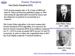
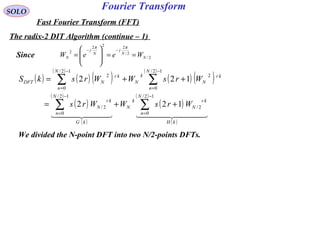
![Fourier TransformSOLO
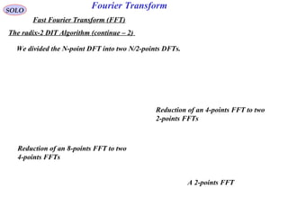
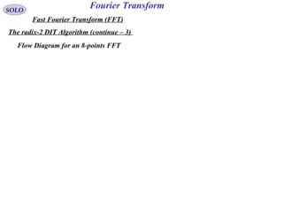
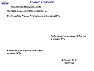
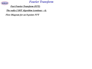
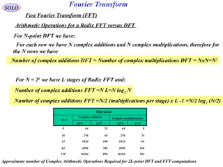
Fast Fourier Transform (FFT)
The radix-2 DIT Algorithm
The radix-2 decimation-in-time (DIT) FFT is the simplest and most common form of the
Cooley-Tukey algorithm, although highly optimized Cooley-Tukey implementations
typically use other forms of the algorithm as described below. Radix-2 DIT divides a DFT
of size N into two interleaved DFTs (hence the name "radix-2") of size N/2 with each
recursive stage.
( ) ( ) ( )∑∑
−
=
−
=
−
==
1
0
1
0
2
:
N
n
nk
s
N
n
nk
N
j
sDFT WTnseTnskS
π
For the sequence s (0), s (Ts),…,s [(N-1) Ts] we define the Discrete Fourier Transform:
1,1, 22/1
2
*
2
+==−====→= −−−
−
ππ
ππ
jNj
evenN
NN
j
N
j
eWeWWeWeW
Suppose N is a power of 2; i.e. N=2L
(L is integer). Since N is a even integer, let compute
SDFT (k) by separate s (nTs) into two (N/2)-point sequences consisting of the even-numbered
points (n=2r) and odd numbered points (n=2r+1).
( ) ( )
( )
( ) ( )
( )
( ) ( )
( )
( ) ( )
( )
∑∑
∑∑
−
=
−
=
−
=
+
−
=
++=
++=
12/
0
2
12/
0
2
12/
0
12
12/
0
2
122
122
N
n
kr
N
k
N
N
n
kr
N
N
n
kr
N
N
n
kr
NDFT
WrsWWrs
WrsWrskS](https://image.slidesharecdn.com/fouriertransform-140924230100-phpapp02/85/Fourier-transform-77-320.jpg)
![Fourier TransformSOLO
Fast Fourier Transform (FFT)
The radix-2 DIT Algorithm (continue – 2)
( ) ( )kkj
kN
N
j
Nk
N eeW 1
2
2/
−==
= −
−
π
π
We divided the N-point DFT into two N/2-points DFTs.
( ) ( ) ( ) ( )
[ ]
( )
( ) ( )
( )
( )
∑∑
−
=
−
−
=
+
++=++=
12/
0
1
2/
12/
0
2/
2/2/
N
n
kn
N
Nk
N
N
n
Nnk
N
kn
NDFT WWNnsnsWNnsWnskS
k
Since N/2 is an even integer (N=2L
)
( ) ( ) ( )[ ]
( )
( )
( )
( )
( )
tgofFFTN
N
n
nl
N
WW
N
N
n
nl
N
ng
DFT WngWNnsnslkS
NN
L
2/
12/
0
2/
2
12/
0
2
2/
2
2/2 ∑∑
−
=
=
=
−
=
=++==
( ) ( ) ( )[ ]
( )
( )
( )
( )
( )
thofFFTN
N
n
nl
N
WW
N
N
n
nl
N
nh
n
NDFT WnhWWNnsnslkS
NN
L
2/
12/
0
2/
2
12/
0
2
2/
2
2/12 ∑∑
−
=
=
=
−
=
=+−=+=](https://image.slidesharecdn.com/fouriertransform-140924230100-phpapp02/85/Fourier-transform-81-320.jpg)
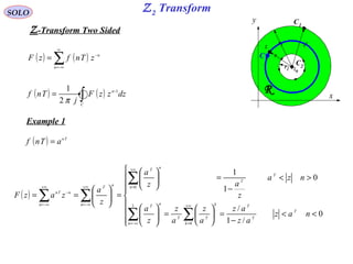
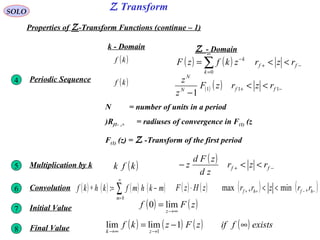
![Z TransformSOLO
Table of Z-Transform Functions
Z - Domain
k - Domain
( )kf ( ) ( ) f
k
k
RzzkfzF >= ∑
∞
=
−
0
1
( )mkf + ( ) ( ) ( ) ( )[ ]110 11
−−−−− +−−
mfzfzfzFz mm
2
( )mkf − ( )zFz m−
3
( ) ( ) ( )kfkfkf −+=∆ 1: ( ) ( ) ( )01 fzzFz −−4
( ) ( ) ( ) ( )kfkfkfkf ++−+=∆ 122:2
( ) ( ) ( ) ( ) ( )1021
2
fzfzzzFz −−−−5
( )kf3
∆ ( ) ( ) ( ) ( ) ( ) ( ) ( )2130331 23
fzfzzfzzzzFz −−−+−−−6](https://image.slidesharecdn.com/fouriertransform-140924230100-phpapp02/85/Fourier-transform-94-320.jpg)


The document provides a detailed explanation of the Fourier Transform, including its properties such as linearity, symmetry, conjugate functions, scaling, derivatives, convolution, and modulation. It presents mathematical proofs and identities related to the Fourier Transform and includes examples of its applications. Additionally, it includes links to visual aids for understanding convolution and signal processing concepts.