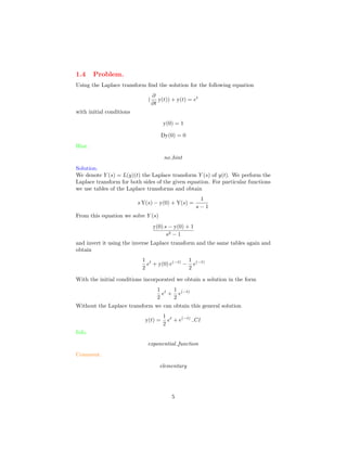
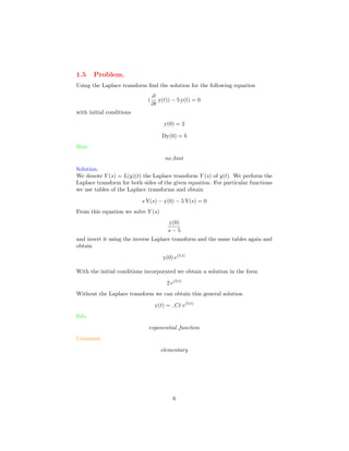
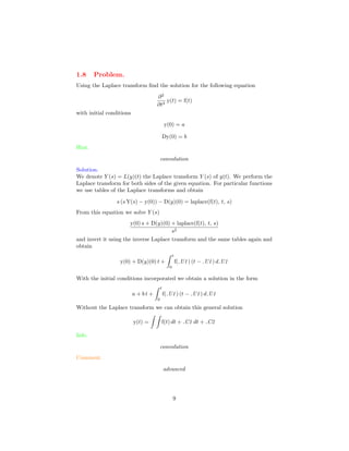
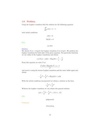
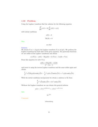
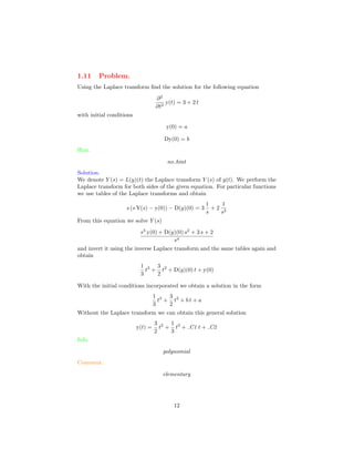
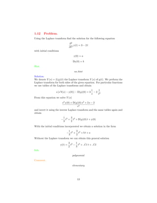
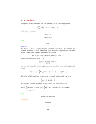
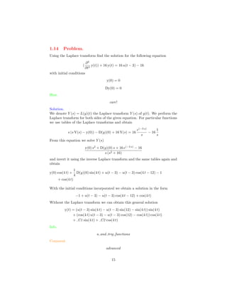
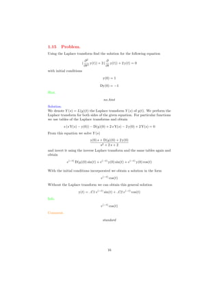
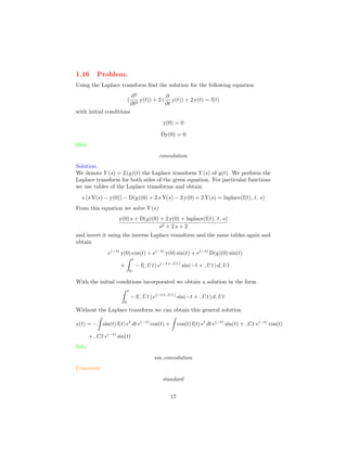
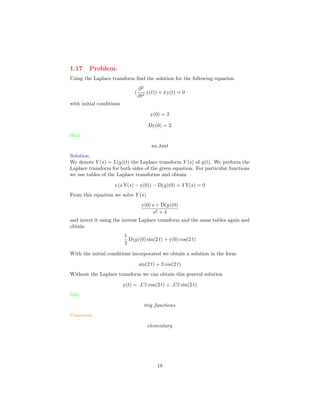
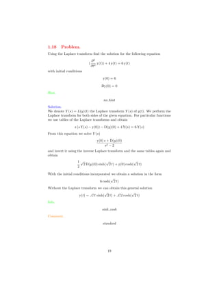
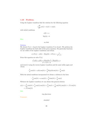
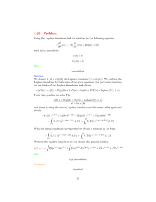
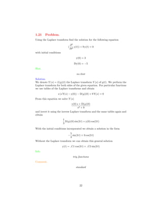
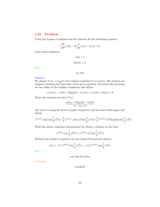
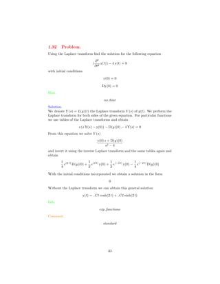
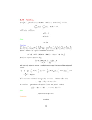
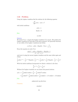
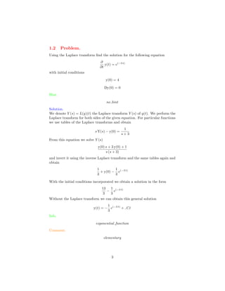
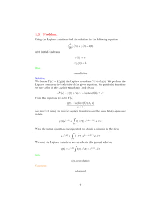
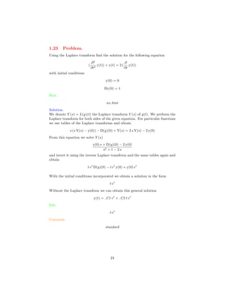
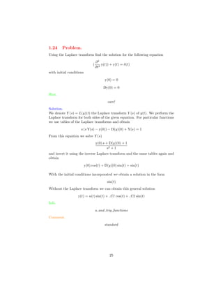
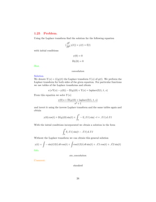
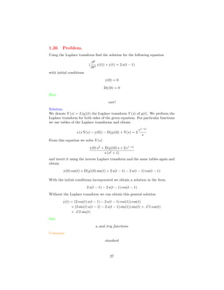
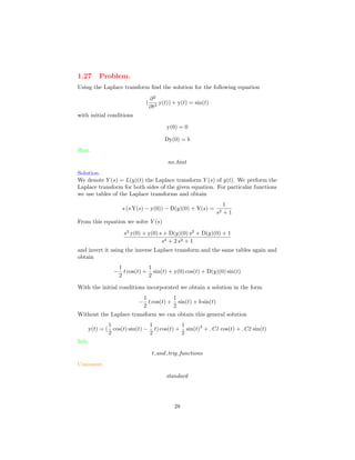
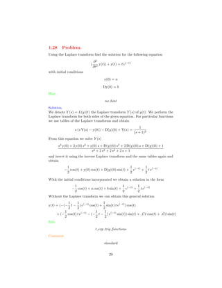
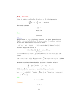
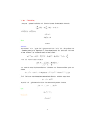
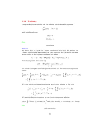
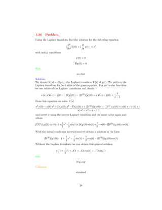
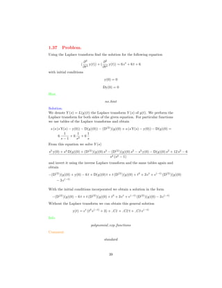
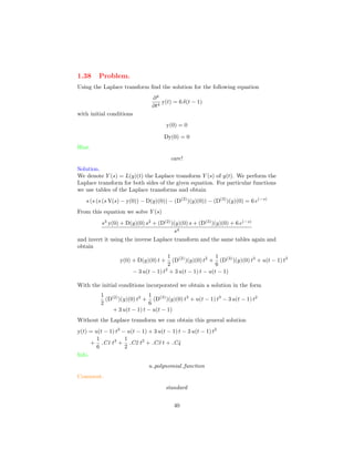
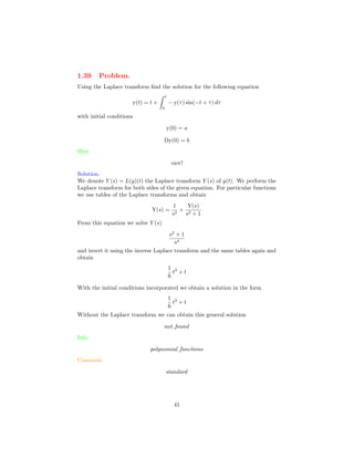
1. The document discusses solving differential equations using the Laplace transform. It provides 13 examples of applying the Laplace transform to find solutions to differential equations with various initial conditions. 2. The examples cover a range of differential equation types, including those with constant coefficients, exponential functions, and polynomials. 3. For each example, the Laplace transform is applied to the differential equation to obtain an expression for the transform Y(s) of the unknown function y(t). This is then inverted using tables of Laplace transforms to find the solution y(t) satisfying the given initial conditions.

1. Laplace Transform
solved problems
Pavel Pyrih
May 24, 2012
( public domain )
Acknowledgement. The following problems were solved using my own procedure
in a program Maple V, release 5, using commands from
Bent E. Petersen: Laplace Transform in Maple
http://people.oregonstate.edu/˜peterseb/mth256/docs/256winter2001 laplace.pdf
All possible errors are my faults.
1 Solving equations using the Laplace transform
Theorem.(Lerch) If two functions have the same integral transform then they
are equal almost everywhere.
This is the right key to the following problems.
Notation.(Dirac & Heaviside) The Dirac unit impuls function will be denoted
by δ(t). The Heaviside step function will be denoted by u(t).
1

2. 1.1 Problem.
Using the Laplace transform find the solution for the following equation
∂
∂t
y(t) = 3 − 2 t
with initial conditions
y(0) = 0
Dy(0) = 0
Hint.
no hint
Solution.
We denote Y (s) = L(y)(t) the Laplace transform Y (s) of y(t). We perform the
Laplace transform for both sides of the given equation. For particular functions
we use tables of the Laplace transforms and obtain
s Y(s) − y(0) = 3
1
s
− 2
1
s2
From this equation we solve Y (s)
y(0) s2
+ 3 s − 2
s3
and invert it using the inverse Laplace transform and the same tables again and
obtain
−t2
+ 3 t + y(0)
With the initial conditions incorporated we obtain a solution in the form
−t2
+ 3 t
Without the Laplace transform we can obtain this general solution
y(t) = −t2
+ 3 t + C1
Info.
polynomial
Comment.
elementary
2

3. 1.2 Problem.
Using the Laplace transform find the solution for the following equation
∂
∂t
y(t) = e(−3 t)
with initial conditions
y(0) = 4
Dy(0) = 0
Hint.
no hint
Solution.
We denote Y (s) = L(y)(t) the Laplace transform Y (s) of y(t). We perform the
Laplace transform for both sides of the given equation. For particular functions
we use tables of the Laplace transforms and obtain
s Y(s) − y(0) =
1
s + 3
From this equation we solve Y (s)
y(0) s + 3 y(0) + 1
s (s + 3)
and invert it using the inverse Laplace transform and the same tables again and
obtain
1
3
+ y(0) −
1
3
e(−3 t)
With the initial conditions incorporated we obtain a solution in the form
13
3
−
1
3
e(−3 t)
Without the Laplace transform we can obtain this general solution
y(t) = −
1
3
e(−3 t)
+ C1
Info.
exponential function
Comment.
elementary
3

4. 1.3 Problem.
Using the Laplace transform find the solution for the following equation
(
∂
∂t
y(t)) + y(t) = f(t)
with initial conditions
y(0) = a
Dy(0) = b
Hint.
convolution
Solution.
We denote Y (s) = L(y)(t) the Laplace transform Y (s) of y(t). We perform the
Laplace transform for both sides of the given equation. For particular functions
we use tables of the Laplace transforms and obtain
s Y(s) − y(0) + Y(s) = laplace(f(t), t, s)
From this equation we solve Y (s)
y(0) + laplace(f(t), t, s)
s + 1
and invert it using the inverse Laplace transform and the same tables again and
obtain
y(0) e(−t)
+
t
0
f( U1) e(−t+ U1)
d U1
With the initial conditions incorporated we obtain a solution in the form
a e(−t)
+
t
0
f( U1) e(−t+ U1)
d U1
Without the Laplace transform we can obtain this general solution
y(t) = e(−t)
f(t) et
dt + e(−t)
C1
Info.
exp convolution
Comment.
advanced
4

5. 1.4 Problem.
Using the Laplace transform find the solution for the following equation
(
∂
∂t
y(t)) + y(t) = et
with initial conditions
y(0) = 1
Dy(0) = 0
Hint.
no hint
Solution.
We denote Y (s) = L(y)(t) the Laplace transform Y (s) of y(t). We perform the
Laplace transform for both sides of the given equation. For particular functions
we use tables of the Laplace transforms and obtain
s Y(s) − y(0) + Y(s) =
1
s − 1
From this equation we solve Y (s)
y(0) s − y(0) + 1
s2 − 1
and invert it using the inverse Laplace transform and the same tables again and
obtain
1
2
et
+ y(0) e(−t)
−
1
2
e(−t)
With the initial conditions incorporated we obtain a solution in the form
1
2
et
+
1
2
e(−t)
Without the Laplace transform we can obtain this general solution
y(t) =
1
2
et
+ e(−t)
C1
Info.
exponential function
Comment.
elementary
5

6. 1.5 Problem.
Using the Laplace transform find the solution for the following equation
(
∂
∂t
y(t)) − 5 y(t) = 0
with initial conditions
y(0) = 2
Dy(0) = b
Hint.
no hint
Solution.
We denote Y (s) = L(y)(t) the Laplace transform Y (s) of y(t). We perform the
Laplace transform for both sides of the given equation. For particular functions
we use tables of the Laplace transforms and obtain
s Y(s) − y(0) − 5 Y(s) = 0
From this equation we solve Y (s)
y(0)
s − 5
and invert it using the inverse Laplace transform and the same tables again and
obtain
y(0) e(5 t)
With the initial conditions incorporated we obtain a solution in the form
2 e(5 t)
Without the Laplace transform we can obtain this general solution
y(t) = C1 e(5 t)
Info.
exponential function
Comment.
elementary
6

7. 1.6 Problem.
Using the Laplace transform find the solution for the following equation
(
∂
∂t
y(t)) − 5 y(t) = e(5 t)
with initial conditions
y(0) = 0
Dy(0) = b
Hint.
no hint
Solution.
We denote Y (s) = L(y)(t) the Laplace transform Y (s) of y(t). We perform the
Laplace transform for both sides of the given equation. For particular functions
we use tables of the Laplace transforms and obtain
s Y(s) − y(0) − 5 Y(s) =
1
s − 5
From this equation we solve Y (s)
y(0) s − 5 y(0) + 1
s2 − 10 s + 25
and invert it using the inverse Laplace transform and the same tables again and
obtain
t e(5 t)
+ y(0) e(5 t)
With the initial conditions incorporated we obtain a solution in the form
t e(5 t)
Without the Laplace transform we can obtain this general solution
y(t) = t e(5 t)
+ C1 e(5 t)
Info.
exponential function
Comment.
elementary
7

8. 1.7 Problem.
Using the Laplace transform find the solution for the following equation
(
∂
∂t
y(t)) − 5 y(t) = e(5 t)
with initial conditions
y(0) = 2
Dy(0) = b
Hint.
no hint
Solution.
We denote Y (s) = L(y)(t) the Laplace transform Y (s) of y(t). We perform the
Laplace transform for both sides of the given equation. For particular functions
we use tables of the Laplace transforms and obtain
s Y(s) − y(0) − 5 Y(s) =
1
s − 5
From this equation we solve Y (s)
y(0) s − 5 y(0) + 1
s2 − 10 s + 25
and invert it using the inverse Laplace transform and the same tables again and
obtain
t e(5 t)
+ y(0) e(5 t)
With the initial conditions incorporated we obtain a solution in the form
t e(5 t)
+ 2 e(5 t)
Without the Laplace transform we can obtain this general solution
y(t) = t e(5 t)
+ C1 e(5 t)
Info.
exponential function
Comment.
elementary
8

9. 1.8 Problem.
Using the Laplace transform find the solution for the following equation
∂2
∂t2
y(t) = f(t)
with initial conditions
y(0) = a
Dy(0) = b
Hint.
convolution
Solution.
We denote Y (s) = L(y)(t) the Laplace transform Y (s) of y(t). We perform the
Laplace transform for both sides of the given equation. For particular functions
we use tables of the Laplace transforms and obtain
s (s Y(s) − y(0)) − D(y)(0) = laplace(f(t), t, s)
From this equation we solve Y (s)
y(0) s + D(y)(0) + laplace(f(t), t, s)
s2
and invert it using the inverse Laplace transform and the same tables again and
obtain
y(0) + D(y)(0) t +
t
0
f( U1) (t − U1) d U1
With the initial conditions incorporated we obtain a solution in the form
a + b t +
t
0
f( U1) (t − U1) d U1
Without the Laplace transform we can obtain this general solution
y(t) = f(t) dt + C1 dt + C2
Info.
convolution
Comment.
advanced
9

10. 1.9 Problem.
Using the Laplace transform find the solution for the following equation
∂2
∂t2
y(t) = 1 − t
with initial conditions
y(0) = 0
Dy(0) = 0
Hint.
no hint
Solution.
We denote Y (s) = L(y)(t) the Laplace transform Y (s) of y(t). We perform the
Laplace transform for both sides of the given equation. For particular functions
we use tables of the Laplace transforms and obtain
s (s Y(s) − y(0)) − D(y)(0) =
1
s
−
1
s2
From this equation we solve Y (s)
s3
y(0) + D(y)(0) s2
+ s − 1
s4
and invert it using the inverse Laplace transform and the same tables again and
obtain
−
1
6
t3
+
1
2
t2
+ D(y)(0) t + y(0)
With the initial conditions incorporated we obtain a solution in the form
−
1
6
t3
+
1
2
t2
Without the Laplace transform we can obtain this general solution
y(t) =
1
2
t2
−
1
6
t3
+ C1 t + C2
Info.
polynomial
Comment.
elementary
10

11. 1.10 Problem.
Using the Laplace transform find the solution for the following equation
∂2
∂t2
y(t) = 2 (
∂
∂t
y(t)) + y(t)
with initial conditions
y(0) = 3
Dy(0) = 6
Hint.
no hint
Solution.
We denote Y (s) = L(y)(t) the Laplace transform Y (s) of y(t). We perform the
Laplace transform for both sides of the given equation. For particular functions
we use tables of the Laplace transforms and obtain
s (s Y(s) − y(0)) − D(y)(0) = 2 s Y(s) − 2 y(0) + Y(s)
From this equation we solve Y (s)
y(0) s + D(y)(0) − 2 y(0)
s2 − 2 s − 1
and invert it using the inverse Laplace transform and the same tables again and
obtain
1
2
et
√
2 D(y)(0) sinh(
√
2 t) −
1
2
et
y(0)
√
2 sinh(
√
2 t) + et
y(0) cosh(
√
2 t)
With the initial conditions incorporated we obtain a solution in the form
3
2
et
√
2 sinh(
√
2 t) + 3 et
cosh(
√
2 t)
Without the Laplace transform we can obtain this general solution
y(t) = C1 e((
√
2+1) t)
+ C2 e(−(
√
2−1) t)
Info.
3 e(2 t)
Comment.
elementary
11

12. 1.11 Problem.
Using the Laplace transform find the solution for the following equation
∂2
∂t2
y(t) = 3 + 2 t
with initial conditions
y(0) = a
Dy(0) = b
Hint.
no hint
Solution.
We denote Y (s) = L(y)(t) the Laplace transform Y (s) of y(t). We perform the
Laplace transform for both sides of the given equation. For particular functions
we use tables of the Laplace transforms and obtain
s (s Y(s) − y(0)) − D(y)(0) = 3
1
s
+ 2
1
s2
From this equation we solve Y (s)
s3
y(0) + D(y)(0) s2
+ 3 s + 2
s4
and invert it using the inverse Laplace transform and the same tables again and
obtain
1
3
t3
+
3
2
t2
+ D(y)(0) t + y(0)
With the initial conditions incorporated we obtain a solution in the form
1
3
t3
+
3
2
t2
+ b t + a
Without the Laplace transform we can obtain this general solution
y(t) =
3
2
t2
+
1
3
t3
+ C1 t + C2
Info.
polynomial
Comment.
elementary
12

13. 1.12 Problem.
Using the Laplace transform find the solution for the following equation
∂2
∂t2
y(t) = 3 − 2 t
with initial conditions
y(0) = a
Dy(0) = b
Hint.
no hint
Solution.
We denote Y (s) = L(y)(t) the Laplace transform Y (s) of y(t). We perform the
Laplace transform for both sides of the given equation. For particular functions
we use tables of the Laplace transforms and obtain
s (s Y(s) − y(0)) − D(y)(0) = 3
1
s
− 2
1
s2
From this equation we solve Y (s)
s3
y(0) + D(y)(0) s2
+ 3 s − 2
s4
and invert it using the inverse Laplace transform and the same tables again and
obtain
−
1
3
t3
+
3
2
t2
+ D(y)(0) t + y(0)
With the initial conditions incorporated we obtain a solution in the form
−
1
3
t3
+
3
2
t2
+ b t + a
Without the Laplace transform we can obtain this general solution
y(t) =
3
2
t2
−
1
3
t3
+ C1 t + C2
Info.
polynomial
Comment.
elementary
13

14. 1.13 Problem.
Using the Laplace transform find the solution for the following equation
(
∂2
∂t2
y(t)) + 16 y(t) = 5 δ(t − 1)
with initial conditions
y(0) = 0
Dy(0) = 0
Hint.
care!
Solution.
We denote Y (s) = L(y)(t) the Laplace transform Y (s) of y(t). We perform the
Laplace transform for both sides of the given equation. For particular functions
we use tables of the Laplace transforms and obtain
s (s Y(s) − y(0)) − D(y)(0) + 16 Y(s) = 5 e(−s)
From this equation we solve Y (s)
y(0) s + D(y)(0) + 5 e(−s)
s2 + 16
and invert it using the inverse Laplace transform and the same tables again and
obtain
y(0) cos(4 t) +
1
4
D(y)(0) sin(4 t) +
5
4
u(t − 1) sin(4 t − 4)
With the initial conditions incorporated we obtain a solution in the form
5
4
u(t − 1) sin(4 t − 4)
Without the Laplace transform we can obtain this general solution
y(t) =
5
4
cos(4) u(t − 1) sin(4 t) −
5
4
sin(4) u(t − 1) cos(4 t) + C1 sin(4 t)
+ C2 cos(4 t)
Info.
u and trig functions
Comment.
advanced
14

15. 1.14 Problem.
Using the Laplace transform find the solution for the following equation
(
∂2
∂t2
y(t)) + 16 y(t) = 16 u(t − 3) − 16
with initial conditions
y(0) = 0
Dy(0) = 0
Hint.
care!
Solution.
We denote Y (s) = L(y)(t) the Laplace transform Y (s) of y(t). We perform the
Laplace transform for both sides of the given equation. For particular functions
we use tables of the Laplace transforms and obtain
s (s Y(s) − y(0)) − D(y)(0) + 16 Y(s) = 16
e(−3 s)
s
− 16
1
s
From this equation we solve Y (s)
y(0) s2
+ D(y)(0) s + 16 e(−3 s)
− 16
s (s2 + 16)
and invert it using the inverse Laplace transform and the same tables again and
obtain
y(0) cos(4 t) +
1
4
D(y)(0) sin(4 t) + u(t − 3) − u(t − 3) cos(4 t − 12) − 1
+ cos(4 t)
With the initial conditions incorporated we obtain a solution in the form
−1 + u(t − 3) − u(t − 3) cos(4 t − 12) + cos(4 t)
Without the Laplace transform we can obtain this general solution
y(t) = (u(t − 3) sin(4 t) − u(t − 3) sin(12) − sin(4 t)) sin(4 t)
+ (cos(4 t) u(t − 3) − u(t − 3) cos(12) − cos(4 t)) cos(4 t)
+ C1 sin(4 t) + C2 cos(4 t)
Info.
u and trig functions
Comment.
advanced
15

16. 1.15 Problem.
Using the Laplace transform find the solution for the following equation
(
∂2
∂t2
y(t)) + 2 (
∂
∂t
y(t)) + 2 y(t) = 0
with initial conditions
y(0) = 1
Dy(0) = −1
Hint.
no hint
Solution.
We denote Y (s) = L(y)(t) the Laplace transform Y (s) of y(t). We perform the
Laplace transform for both sides of the given equation. For particular functions
we use tables of the Laplace transforms and obtain
s (s Y(s) − y(0)) − D(y)(0) + 2 s Y(s) − 2 y(0) + 2 Y(s) = 0
From this equation we solve Y (s)
y(0) s + D(y)(0) + 2 y(0)
s2 + 2 s + 2
and invert it using the inverse Laplace transform and the same tables again and
obtain
e(−t)
D(y)(0) sin(t) + e(−t)
y(0) sin(t) + e(−t)
y(0) cos(t)
With the initial conditions incorporated we obtain a solution in the form
e(−t)
cos(t)
Without the Laplace transform we can obtain this general solution
y(t) = C1 e(−t)
sin(t) + C2 e(−t)
cos(t)
Info.
e(−t)
cos(t)
Comment.
standard
16

17. 1.16 Problem.
Using the Laplace transform find the solution for the following equation
(
∂2
∂t2
y(t)) + 2 (
∂
∂t
y(t)) + 2 y(t) = f(t)
with initial conditions
y(0) = 0
Dy(0) = 0
Hint.
convolution
Solution.
We denote Y (s) = L(y)(t) the Laplace transform Y (s) of y(t). We perform the
Laplace transform for both sides of the given equation. For particular functions
we use tables of the Laplace transforms and obtain
s (s Y(s) − y(0)) − D(y)(0) + 2 s Y(s) − 2 y(0) + 2 Y(s) = laplace(f(t), t, s)
From this equation we solve Y (s)
y(0) s + D(y)(0) + 2 y(0) + laplace(f(t), t, s)
s2 + 2 s + 2
and invert it using the inverse Laplace transform and the same tables again and
obtain
e(−t)
y(0) cos(t) + e(−t)
y(0) sin(t) + e(−t)
D(y)(0) sin(t)
+
t
0
− f( U1) e(−t+ U1)
sin(−t + U1) d U1
With the initial conditions incorporated we obtain a solution in the form
t
0
− f( U1) e(−t+ U1)
sin(−t + U1) d U1
Without the Laplace transform we can obtain this general solution
y(t) = − sin(t) f(t) et
dt e(−t)
cos(t) + cos(t) f(t) et
dt e(−t)
sin(t) + C1 e(−t)
cos(t)
+ C2 e(−t)
sin(t)
Info.
sin convolution
Comment.
standard
17

18. 1.17 Problem.
Using the Laplace transform find the solution for the following equation
(
∂2
∂t2
y(t)) + 4 y(t) = 0
with initial conditions
y(0) = 2
Dy(0) = 2
Hint.
no hint
Solution.
We denote Y (s) = L(y)(t) the Laplace transform Y (s) of y(t). We perform the
Laplace transform for both sides of the given equation. For particular functions
we use tables of the Laplace transforms and obtain
s (s Y(s) − y(0)) − D(y)(0) + 4 Y(s) = 0
From this equation we solve Y (s)
y(0) s + D(y)(0)
s2 + 4
and invert it using the inverse Laplace transform and the same tables again and
obtain
1
2
D(y)(0) sin(2 t) + y(0) cos(2 t)
With the initial conditions incorporated we obtain a solution in the form
sin(2 t) + 2 cos(2 t)
Without the Laplace transform we can obtain this general solution
y(t) = C1 cos(2 t) + C2 sin(2 t)
Info.
trig functions
Comment.
elementary
18

19. 1.18 Problem.
Using the Laplace transform find the solution for the following equation
(
∂2
∂t2
y(t)) + 4 y(t) = 6 y(t)
with initial conditions
y(0) = 6
Dy(0) = 0
Hint.
no hint
Solution.
We denote Y (s) = L(y)(t) the Laplace transform Y (s) of y(t). We perform the
Laplace transform for both sides of the given equation. For particular functions
we use tables of the Laplace transforms and obtain
s (s Y(s) − y(0)) − D(y)(0) + 4 Y(s) = 6 Y(s)
From this equation we solve Y (s)
y(0) s + D(y)(0)
s2 − 2
and invert it using the inverse Laplace transform and the same tables again and
obtain
1
2
√
2 D(y)(0) sinh(
√
2 t) + y(0) cosh(
√
2 t)
With the initial conditions incorporated we obtain a solution in the form
6 cosh(
√
2 t)
Without the Laplace transform we can obtain this general solution
y(t) = C1 sinh(
√
2 t) + C2 cosh(
√
2 t)
Info.
sinh cosh
Comment.
standard
19

20. 1.19 Problem.
Using the Laplace transform find the solution for the following equation
(
∂2
∂t2
y(t)) + 4 y(t) = cos(t)
with initial conditions
y(0) = a
Dy(0) = b
Hint.
no hint
Solution.
We denote Y (s) = L(y)(t) the Laplace transform Y (s) of y(t). We perform the
Laplace transform for both sides of the given equation. For particular functions
we use tables of the Laplace transforms and obtain
s (s Y(s) − y(0)) − D(y)(0) + 4 Y(s) =
s
s2 + 1
From this equation we solve Y (s)
s3
y(0) + y(0) s + D(y)(0) s2
+ D(y)(0) + s
s4 + 5 s2 + 4
and invert it using the inverse Laplace transform and the same tables again and
obtain
−
1
3
cos(2 t) + y(0) cos(2 t) +
1
2
D(y)(0) sin(2 t) +
1
3
cos(t)
With the initial conditions incorporated we obtain a solution in the form
−
1
3
cos(2 t) + a cos(2 t) +
1
2
b sin(2 t) +
1
3
cos(t)
Without the Laplace transform we can obtain this general solution
y(t) = (
1
12
cos(3 t) +
1
4
cos(t)) cos(2 t) + (
1
4
sin(t) +
1
12
sin(3 t)) sin(2 t) + C1 cos(2 t)
+ C2 sin(2 t)
Info.
trig functions
Comment.
standard
20

21. 1.20 Problem.
Using the Laplace transform find the solution for the following equation
(
∂2
∂t2
y(t)) + 9 (
∂
∂t
y(t)) + 20 y(t) = f(t)
with initial conditions
y(0) = 0
Dy(0) = 0
Hint.
convolution
Solution.
We denote Y (s) = L(y)(t) the Laplace transform Y (s) of y(t). We perform the
Laplace transform for both sides of the given equation. For particular functions
we use tables of the Laplace transforms and obtain
s (s Y(s) − y(0)) − D(y)(0) + 9 s Y(s) − 9 y(0) + 20 Y(s) = laplace(f(t), t, s)
From this equation we solve Y (s)
y(0) s + D(y)(0) + 9 y(0) + laplace(f(t), t, s)
s2 + 9 s + 20
and invert it using the inverse Laplace transform and the same tables again and
obtain
−4 y(0) e(−5 t)
+ 5 y(0) e(−4 t)
− D(y)(0) e(−5 t)
+ D(y)(0) e(−4 t)
−
t
0
f( U1) e(−5 t+5 U1)
d U1 +
t
0
f( U2) e(−4 t+4 U2)
d U2
With the initial conditions incorporated we obtain a solution in the form
−
t
0
f( U1) e(−5 t+5 U1)
d U1 +
t
0
f( U2) e(−4 t+4 U2)
d U2
Without the Laplace transform we can obtain this general solution
y(t) = −(− f(t) e(4 t)
dt e(5 t)
+ f(t) e(5 t)
dt e(4 t)
) e(−9 t)
+ C1 e(−4 t)
+ C2 e(−5 t)
Info.
exp convolution
Comment.
standard
21

22. 1.21 Problem.
Using the Laplace transform find the solution for the following equation
(
∂2
∂t2
y(t)) + 9 y(t) = 0
with initial conditions
y(0) = 3
Dy(0) = −5
Hint.
no hint
Solution.
We denote Y (s) = L(y)(t) the Laplace transform Y (s) of y(t). We perform the
Laplace transform for both sides of the given equation. For particular functions
we use tables of the Laplace transforms and obtain
s (s Y(s) − y(0)) − D(y)(0) + 9 Y(s) = 0
From this equation we solve Y (s)
y(0) s + D(y)(0)
s2 + 9
and invert it using the inverse Laplace transform and the same tables again and
obtain
1
3
D(y)(0) sin(3 t) + y(0) cos(3 t)
With the initial conditions incorporated we obtain a solution in the form
−
5
3
sin(3 t) + 3 cos(3 t)
Without the Laplace transform we can obtain this general solution
y(t) = C1 cos(3 t) + C2 sin(3 t)
Info.
trig functions
Comment.
standard
22

23. 1.22 Problem.
Using the Laplace transform find the solution for the following equation
(
∂2
∂t2
y(t)) + y(t) = 0
with initial conditions
y(0) = 0
Dy(0) = 1
Hint.
no hint
Solution.
We denote Y (s) = L(y)(t) the Laplace transform Y (s) of y(t). We perform the
Laplace transform for both sides of the given equation. For particular functions
we use tables of the Laplace transforms and obtain
s (s Y(s) − y(0)) − D(y)(0) + Y(s) = 0
From this equation we solve Y (s)
y(0) s + D(y)(0)
s2 + 1
and invert it using the inverse Laplace transform and the same tables again and
obtain
y(0) cos(t) + D(y)(0) sin(t)
With the initial conditions incorporated we obtain a solution in the form
sin(t)
Without the Laplace transform we can obtain this general solution
y(t) = C1 cos(t) + C2 sin(t)
Info.
trig functions
Comment.
standard
23

24. 1.23 Problem.
Using the Laplace transform find the solution for the following equation
(
∂2
∂t2
y(t)) + y(t) = 2 (
∂
∂t
y(t))
with initial conditions
y(0) = 0
Dy(0) = 1
Hint.
no hint
Solution.
We denote Y (s) = L(y)(t) the Laplace transform Y (s) of y(t). We perform the
Laplace transform for both sides of the given equation. For particular functions
we use tables of the Laplace transforms and obtain
s (s Y(s) − y(0)) − D(y)(0) + Y(s) = 2 s Y(s) − 2 y(0)
From this equation we solve Y (s)
y(0) s + D(y)(0) − 2 y(0)
s2 + 1 − 2 s
and invert it using the inverse Laplace transform and the same tables again and
obtain
t et
D(y)(0) − t et
y(0) + y(0) et
With the initial conditions incorporated we obtain a solution in the form
t et
Without the Laplace transform we can obtain this general solution
y(t) = C1 et
+ C2 t et
Info.
t et
Comment.
standard
24

25. 1.24 Problem.
Using the Laplace transform find the solution for the following equation
(
∂2
∂t2
y(t)) + y(t) = δ(t)
with initial conditions
y(0) = 0
Dy(0) = 0
Hint.
care!
Solution.
We denote Y (s) = L(y)(t) the Laplace transform Y (s) of y(t). We perform the
Laplace transform for both sides of the given equation. For particular functions
we use tables of the Laplace transforms and obtain
s (s Y(s) − y(0)) − D(y)(0) + Y(s) = 1
From this equation we solve Y (s)
y(0) s + D(y)(0) + 1
s2 + 1
and invert it using the inverse Laplace transform and the same tables again and
obtain
y(0) cos(t) + D(y)(0) sin(t) + sin(t)
With the initial conditions incorporated we obtain a solution in the form
sin(t)
Without the Laplace transform we can obtain this general solution
y(t) = u(t) sin(t) + C1 cos(t) + C2 sin(t)
Info.
u and trig functions
Comment.
standard
25

26. 1.25 Problem.
Using the Laplace transform find the solution for the following equation
(
∂2
∂t2
y(t)) + y(t) = f(t)
with initial conditions
y(0) = 0
Dy(0) = 0
Hint.
convolution
Solution.
We denote Y (s) = L(y)(t) the Laplace transform Y (s) of y(t). We perform the
Laplace transform for both sides of the given equation. For particular functions
we use tables of the Laplace transforms and obtain
s (s Y(s) − y(0)) − D(y)(0) + Y(s) = laplace(f(t), t, s)
From this equation we solve Y (s)
y(0) s + D(y)(0) + laplace(f(t), t, s)
s2 + 1
and invert it using the inverse Laplace transform and the same tables again and
obtain
y(0) cos(t) + D(y)(0) sin(t) +
t
0
− f( U1) sin(−t + U1) d U1
With the initial conditions incorporated we obtain a solution in the form
t
0
f( U1) sin(t − U1) d U1
Without the Laplace transform we can obtain this general solution
y(t) = − sin(t) f(t) dt cos(t) + cos(t) f(t) dt sin(t) + C1 cos(t) + C2 sin(t)
Info.
sin convolution
Comment.
standard
26

27. 1.26 Problem.
Using the Laplace transform find the solution for the following equation
(
∂2
∂t2
y(t)) + y(t) = 2 u(t − 1)
with initial conditions
y(0) = 0
Dy(0) = 0
Hint.
care!
Solution.
We denote Y (s) = L(y)(t) the Laplace transform Y (s) of y(t). We perform the
Laplace transform for both sides of the given equation. For particular functions
we use tables of the Laplace transforms and obtain
s (s Y(s) − y(0)) − D(y)(0) + Y(s) = 2
e(−s)
s
From this equation we solve Y (s)
y(0) s2
+ D(y)(0) s + 2 e(−s)
s (s2 + 1)
and invert it using the inverse Laplace transform and the same tables again and
obtain
y(0) cos(t) + D(y)(0) sin(t) + 2 u(t − 1) − 2 u(t − 1) cos(t − 1)
With the initial conditions incorporated we obtain a solution in the form
2 u(t − 1) − 2 u(t − 1) cos(t − 1)
Without the Laplace transform we can obtain this general solution
y(t) = (2 cos(t) u(t − 1) − 2 u(t − 1) cos(1)) cos(t)
+ (2 sin(t) u(t − 1) − 2 u(t − 1) sin(1)) sin(t) + C1 cos(t)
+ C2 sin(t)
Info.
u and trig functions
Comment.
standard
27

28. 1.27 Problem.
Using the Laplace transform find the solution for the following equation
(
∂2
∂t2
y(t)) + y(t) = sin(t)
with initial conditions
y(0) = 0
Dy(0) = b
Hint.
no hint
Solution.
We denote Y (s) = L(y)(t) the Laplace transform Y (s) of y(t). We perform the
Laplace transform for both sides of the given equation. For particular functions
we use tables of the Laplace transforms and obtain
s (s Y(s) − y(0)) − D(y)(0) + Y(s) =
1
s2 + 1
From this equation we solve Y (s)
s3
y(0) + y(0) s + D(y)(0) s2
+ D(y)(0) + 1
s4 + 2 s2 + 1
and invert it using the inverse Laplace transform and the same tables again and
obtain
−
1
2
t cos(t) +
1
2
sin(t) + y(0) cos(t) + D(y)(0) sin(t)
With the initial conditions incorporated we obtain a solution in the form
−
1
2
t cos(t) +
1
2
sin(t) + b sin(t)
Without the Laplace transform we can obtain this general solution
y(t) = (
1
2
cos(t) sin(t) −
1
2
t) cos(t) +
1
2
sin(t)3
+ C1 cos(t) + C2 sin(t)
Info.
t and trig functions
Comment.
standard
28

29. 1.28 Problem.
Using the Laplace transform find the solution for the following equation
(
∂2
∂t2
y(t)) + y(t) = t e(−t)
with initial conditions
y(0) = a
Dy(0) = b
Hint.
no hint
Solution.
We denote Y (s) = L(y)(t) the Laplace transform Y (s) of y(t). We perform the
Laplace transform for both sides of the given equation. For particular functions
we use tables of the Laplace transforms and obtain
s (s Y(s) − y(0)) − D(y)(0) + Y(s) =
1
(s + 1)2
From this equation we solve Y (s)
s3
y(0) + 2 y(0) s2
+ y(0) s + D(y)(0) s2
+ 2 D(y)(0) s + D(y)(0) + 1
s4 + 2 s3 + 2 s2 + 2 s + 1
and invert it using the inverse Laplace transform and the same tables again and
obtain
−
1
2
cos(t) + y(0) cos(t) + D(y)(0) sin(t) +
1
2
e(−t)
+
1
2
t e(−t)
With the initial conditions incorporated we obtain a solution in the form
−
1
2
cos(t) + a cos(t) + b sin(t) +
1
2
e(−t)
+
1
2
t e(−t)
Without the Laplace transform we can obtain this general solution
y(t) = (−(−
1
2
t −
1
2
) e(−t)
cos(t) +
1
2
sin(t) t e(−t)
) cos(t)
+ (−
1
2
cos(t) t e(−t)
− (−
1
2
t −
1
2
) e(−t)
sin(t)) sin(t) + C1 cos(t) + C2 sin(t)
Info.
t exp trig functions
Comment.
standard
29

30. 1.29 Problem.
Using the Laplace transform find the solution for the following equation
(
∂2
∂t2
y(t)) − 2 (
∂
∂t
y(t)) + 2 y(t) = f(t)
with initial conditions
y(0) = 0
Dy(0) = 0
Hint.
convolution
Solution.
We denote Y (s) = L(y)(t) the Laplace transform Y (s) of y(t). We perform the
Laplace transform for both sides of the given equation. For particular functions
we use tables of the Laplace transforms and obtain
s (s Y(s) − y(0)) − D(y)(0) − 2 s Y(s) + 2 y(0) + 2 Y(s) = laplace(f(t), t, s)
From this equation we solve Y (s)
y(0) s + D(y)(0) − 2 y(0) + laplace(f(t), t, s)
s2 − 2 s + 2
and invert it using the inverse Laplace transform and the same tables again and
obtain
y(0) et
cos(t)−y(0) et
sin(t)+D(y)(0) et
sin(t)+
t
0
−f( U1) e(t− U1)
sin(−t+ U1) d U1
With the initial conditions incorporated we obtain a solution in the form
t
0
− f( U1) e(t− U1)
sin(−t + U1) d U1
Without the Laplace transform we can obtain this general solution
y(t) = −(− cos(t) f(t) e(−t)
dt sin(t) + sin(t) f(t) e(−t)
dt cos(t)) et
+ C1 et
sin(t)
+ C2 et
cos(t)
Info.
sin exp convolution
Comment.
standard
30

31. 1.30 Problem.
Using the Laplace transform find the solution for the following equation
(
∂2
∂t2
y(t)) − 3 (
∂
∂t
y(t)) + 2 y(t) = 4
with initial conditions
y(0) = 2
Dy(0) = 3
Hint.
no hint
Solution.
We denote Y (s) = L(y)(t) the Laplace transform Y (s) of y(t). We perform the
Laplace transform for both sides of the given equation. For particular functions
we use tables of the Laplace transforms and obtain
s (s Y(s) − y(0)) − D(y)(0) − 3 s Y(s) + 3 y(0) + 2 Y(s) = 4
1
s
From this equation we solve Y (s)
y(0) s2
+ D(y)(0) s − 3 y(0) s + 4
s (s2 − 3 s + 2)
and invert it using the inverse Laplace transform and the same tables again and
obtain
2 − 4 et
+ 2 y(0) et
− et
D(y)(0) + 2 e(2 t)
− e(2 t)
y(0) + e(2 t)
D(y)(0)
With the initial conditions incorporated we obtain a solution in the form
2 − 3 et
+ 3 e(2 t)
Without the Laplace transform we can obtain this general solution
y(t) = 2 + C1 et
+ C2 e(2 t)
Info.
exp functions
Comment.
standard
31

32. 1.31 Problem.
Using the Laplace transform find the solution for the following equation
(
∂2
∂t2
y(t)) − 3 (
∂
∂t
y(t)) + 4 y(t) = 0
with initial conditions
y(0) = 1
Dy(0) = 5
Hint.
no hint
Solution.
We denote Y (s) = L(y)(t) the Laplace transform Y (s) of y(t). We perform the
Laplace transform for both sides of the given equation. For particular functions
we use tables of the Laplace transforms and obtain
s (s Y(s) − y(0)) − D(y)(0) − 3 s Y(s) + 3 y(0) + 4 Y(s) = 0
From this equation we solve Y (s)
y(0) s + D(y)(0) − 3 y(0)
s2 − 3 s + 4
and invert it using the inverse Laplace transform and the same tables again and
obtain
e(3/2 t)
y(0) cos(
1
2
√
7 t)−
3
7
e(3/2 t)
y(0)
√
7 sin(
1
2
√
7 t)+
2
7
e(3/2 t)
√
7 D(y)(0) sin(
1
2
√
7 t)
With the initial conditions incorporated we obtain a solution in the form
e(3/2 t)
cos(
1
2
√
7 t) + e(3/2 t)
√
7 sin(
1
2
√
7 t)
Without the Laplace transform we can obtain this general solution
y(t) = C1 e(3/2 t)
sin(
1
2
√
7 t) + C2 e(3/2 t)
cos(
1
2
√
7 t)
Info.
exp trig functions
Comment.
standard
32

33. 1.32 Problem.
Using the Laplace transform find the solution for the following equation
(
∂2
∂t2
y(t)) − 4 y(t) = 0
with initial conditions
y(0) = 0
Dy(0) = 0
Hint.
no hint
Solution.
We denote Y (s) = L(y)(t) the Laplace transform Y (s) of y(t). We perform the
Laplace transform for both sides of the given equation. For particular functions
we use tables of the Laplace transforms and obtain
s (s Y(s) − y(0)) − D(y)(0) − 4 Y(s) = 0
From this equation we solve Y (s)
y(0) s + D(y)(0)
s2 − 4
and invert it using the inverse Laplace transform and the same tables again and
obtain
1
4
e(2 t)
D(y)(0) +
1
2
e(2 t)
y(0) +
1
2
e(−2 t)
y(0) −
1
4
e(−2 t)
D(y)(0)
With the initial conditions incorporated we obtain a solution in the form
0
Without the Laplace transform we can obtain this general solution
y(t) = C1 cosh(2 t) + C2 sinh(2 t)
Info.
exp functions
Comment.
standard
33

34. 1.33 Problem.
Using the Laplace transform find the solution for the following equation
(
∂2
∂t2
y(t)) − (
∂
∂t
y(t)) − 2 y(t) = 4 t2
with initial conditions
y(0) = 1
Dy(0) = 4
Hint.
no hint
Solution.
We denote Y (s) = L(y)(t) the Laplace transform Y (s) of y(t). We perform the
Laplace transform for both sides of the given equation. For particular functions
we use tables of the Laplace transforms and obtain
s (s Y(s) − y(0)) − D(y)(0) − s Y(s) + y(0) − 2 Y(s) = 8
1
s3
From this equation we solve Y (s)
s4
y(0) + D(y)(0) s3
− s3
y(0) + 8
s3 (s2 − s − 2)
and invert it using the inverse Laplace transform and the same tables again and
obtain
−3 + 2 t − 2 t2
+
8
3
e(−t)
+
2
3
y(0) e(−t)
−
1
3
e(−t)
D(y)(0) +
1
3
e(2 t)
y(0) +
1
3
e(2 t)
+
1
3
e(2 t)
D(y)(0)
With the initial conditions incorporated we obtain a solution in the form
−3 + 2 t − 2 t2
+ 2 e(−t)
+ 2 e(2 t)
Without the Laplace transform we can obtain this general solution
y(t) = −3 + 2 t − 2 t2
+ C1 e(2 t)
+ C2 e(−t)
Info.
polynomial exp functions
Comment.
standard
34

35. 1.34 Problem.
Using the Laplace transform find the solution for the following equation
(
∂2
∂t2
y(t)) − y(t) = et
with initial conditions
y(0) = 1
Dy(0) = 0
Hint.
no hint
Solution.
We denote Y (s) = L(y)(t) the Laplace transform Y (s) of y(t). We perform the
Laplace transform for both sides of the given equation. For particular functions
we use tables of the Laplace transforms and obtain
s (s Y(s) − y(0)) − D(y)(0) − Y(s) =
1
s − 1
From this equation we solve Y (s)
y(0) s2
− y(0) s + D(y)(0) s − D(y)(0) + 1
s3 − s2 − s + 1
and invert it using the inverse Laplace transform and the same tables again and
obtain
1
2
y(0) e(−t)
−
1
2
e(−t)
D(y)(0) +
1
4
e(−t)
+
1
2
y(0) et
+
1
2
et
D(y)(0) −
1
4
et
+
1
2
t et
With the initial conditions incorporated we obtain a solution in the form
3
4
e(−t)
+
1
4
et
+
1
2
t et
Without the Laplace transform we can obtain this general solution
y(t) = (−
1
2
sinh(t) cosh(t) +
1
2
t −
1
2
cosh(t)2
) cosh(t)
+ (
1
2
cosh(t)2
+
1
2
sinh(t) cosh(t) +
1
2
t) sinh(t) + C1 cosh(t) + C2 sinh(t)
Info.
polynomial exp functions
Comment.
standard
35

36. 1.35 Problem.
Using the Laplace transform find the solution for the following equation
(
∂2
∂t2
y(t)) − y(t) = f(t)
with initial conditions
y(0) = a
Dy(0) = b
Hint.
convolution
Solution.
We denote Y (s) = L(y)(t) the Laplace transform Y (s) of y(t). We perform the
Laplace transform for both sides of the given equation. For particular functions
we use tables of the Laplace transforms and obtain
s (s Y(s) − y(0)) − D(y)(0) − Y(s) = laplace(f(t), t, s)
From this equation we solve Y (s)
y(0) s + D(y)(0) + laplace(f(t), t, s)
s2 − 1
and invert it using the inverse Laplace transform and the same tables again and
obtain
1
2
y(0) et
+
1
2
y(0) e(−t)
+
1
2
et
D(y)(0) −
1
2
e(−t)
D(y)(0) +
1
2
t
0
f( U1) e(t− U1)
d U1
−
1
2
t
0
f( U2) e(−t+ U2)
d U2
With the initial conditions incorporated we obtain a solution in the form
1
2
a et
+
1
2
a e(−t)
+
1
2
et
b −
1
2
e(−t)
b +
1
2
t
0
f( U1) e(t− U1)
d U1
−
1
2
t
0
f( U2) e(−t+ U2)
d U2
Without the Laplace transform we can obtain this general solution
y(t) = −sinh(t) f(t) dt cosh(t)+ cosh(t) f(t) dt sinh(t)+ C1 cosh(t)+ C2 sinh(t)
Info.
exp convolution
36

37. Comment.
standard
37

38. 1.36 Problem.
Using the Laplace transform find the solution for the following equation
(
∂3
∂t3
y(t)) + (
∂
∂t
y(t)) = et
with initial conditions
y(0) = 0
Dy(0) = 0
Hint.
no hint
Solution.
We denote Y (s) = L(y)(t) the Laplace transform Y (s) of y(t). We perform the
Laplace transform for both sides of the given equation. For particular functions
we use tables of the Laplace transforms and obtain
s (s (s Y(s) − y(0)) − D(y)(0)) − (D(2)
)(y)(0) + s Y(s) − y(0) =
1
s − 1
From this equation we solve Y (s)
s3
y(0) − y(0) s2
+ D(y)(0) s2
− D(y)(0) s + (D(2)
)(y)(0) s − (D(2)
)(y)(0) + y(0) s − y(0) + 1
s (s3 − s2 + s − 1)
and invert it using the inverse Laplace transform and the same tables again and
obtain
(D(2)
)(y)(0)+y(0)−1+
1
2
et
−
1
2
sin(t)+D(y)(0) sin(t)+
1
2
cos(t)−(D(2)
)(y)(0) cos(t)
With the initial conditions incorporated we obtain a solution in the form
(D(2)
)(y)(0) − 1 +
1
2
et
−
1
2
sin(t) +
1
2
cos(t) − (D(2)
)(y)(0) cos(t)
Without the Laplace transform we can obtain this general solution
y(t) =
1
2
et
+ C1 + C2 cos(t) + C3 sin(t)
Info.
trig exp
Comment.
standard
38

39. 1.37 Problem.
Using the Laplace transform find the solution for the following equation
(
∂3
∂t3
y(t)) + (
∂2
∂t2
y(t)) = 6 et
+ 6 t + 6
with initial conditions
y(0) = 0
Dy(0) = 0
Hint.
no hint
Solution.
We denote Y (s) = L(y)(t) the Laplace transform Y (s) of y(t). We perform the
Laplace transform for both sides of the given equation. For particular functions
we use tables of the Laplace transforms and obtain
s (s (s Y(s) − y(0)) − D(y)(0)) − (D(2)
)(y)(0) + s (s Y(s) − y(0)) − D(y)(0) =
6
1
s − 1
+ 6
1
s2
+ 6
1
s
From this equation we solve Y (s)
s5
y(0) + s4
D(y)(0) + (D(2)
)(y)(0) s3
− (D(2)
)(y)(0) s2
− s3
y(0) − D(y)(0) s2
+ 12 s2
− 6
s4 (s2 − 1)
and invert it using the inverse Laplace transform and the same tables again and
obtain
−(D(2)
)(y)(0) + y(0) − 6 t + D(y)(0) t + t (D(2)
)(y)(0) + t3
+ 3 et
+ e(−t)
(D(2)
)(y)(0)
− 3 e(−t)
With the initial conditions incorporated we obtain a solution in the form
−(D(2)
)(y)(0) − 6 t + t (D(2)
)(y)(0) + t3
+ 3 et
+ e(−t)
(D(2)
)(y)(0) − 3 e(−t)
Without the Laplace transform we can obtain this general solution
y(t) = et
(t3
e(−t)
+ 3) + C1 + C2 t + C3 e(−t)
Info.
polynomial exp functions
Comment.
standard
39

40. 1.38 Problem.
Using the Laplace transform find the solution for the following equation
∂4
∂t4
y(t) = 6 δ(t − 1)
with initial conditions
y(0) = 0
Dy(0) = 0
Hint.
care!
Solution.
We denote Y (s) = L(y)(t) the Laplace transform Y (s) of y(t). We perform the
Laplace transform for both sides of the given equation. For particular functions
we use tables of the Laplace transforms and obtain
s (s (s (s Y(s) − y(0)) − D(y)(0)) − (D(2)
)(y)(0)) − (D(3)
)(y)(0) = 6 e(−s)
From this equation we solve Y (s)
s3
y(0) + D(y)(0) s2
+ (D(2)
)(y)(0) s + (D(3)
)(y)(0) + 6 e(−s)
s4
and invert it using the inverse Laplace transform and the same tables again and
obtain
y(0) + D(y)(0) t +
1
2
(D(2)
)(y)(0) t2
+
1
6
(D(3)
)(y)(0) t3
+ u(t − 1) t3
− 3 u(t − 1) t2
+ 3 u(t − 1) t − u(t − 1)
With the initial conditions incorporated we obtain a solution in the form
1
2
(D(2)
)(y)(0) t2
+
1
6
(D(3)
)(y)(0) t3
+ u(t − 1) t3
− 3 u(t − 1) t2
+ 3 u(t − 1) t − u(t − 1)
Without the Laplace transform we can obtain this general solution
y(t) = u(t − 1) t3
− u(t − 1) + 3 u(t − 1) t − 3 u(t − 1) t2
+
1
6
C1 t3
+
1
2
C2 t2
+ C3 t + C4
Info.
u polynomial function
Comment.
standard
40

41. 1.39 Problem.
Using the Laplace transform find the solution for the following equation
y(t) = t +
t
0
− y(τ) sin(−t + τ) dτ
with initial conditions
y(0) = a
Dy(0) = b
Hint.
care!
Solution.
We denote Y (s) = L(y)(t) the Laplace transform Y (s) of y(t). We perform the
Laplace transform for both sides of the given equation. For particular functions
we use tables of the Laplace transforms and obtain
Y(s) =
1
s2
+
Y(s)
s2 + 1
From this equation we solve Y (s)
s2
+ 1
s4
and invert it using the inverse Laplace transform and the same tables again and
obtain
1
6
t3
+ t
With the initial conditions incorporated we obtain a solution in the form
1
6
t3
+ t
Without the Laplace transform we can obtain this general solution
not found
Info.
polynomial functions
Comment.
standard
41