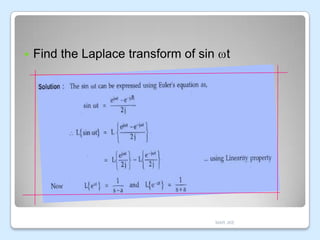
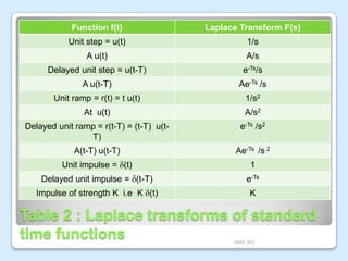
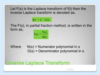
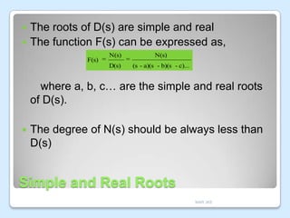
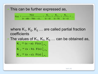
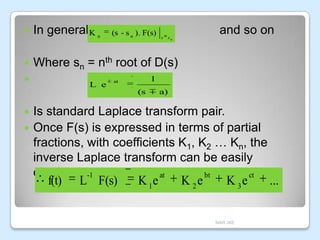
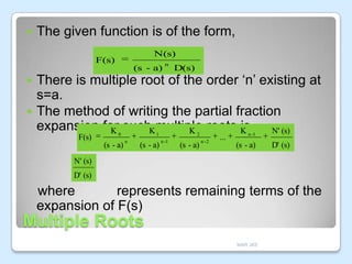
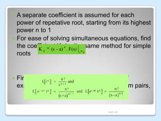
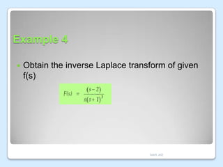
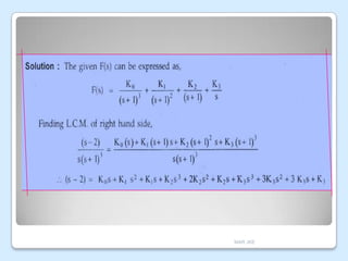
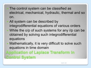
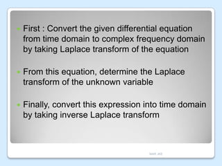
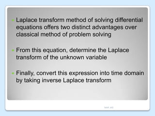
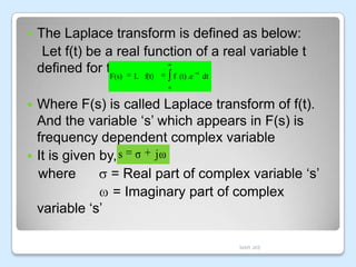
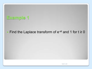
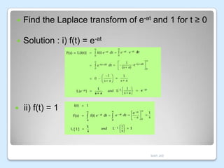
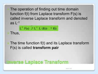
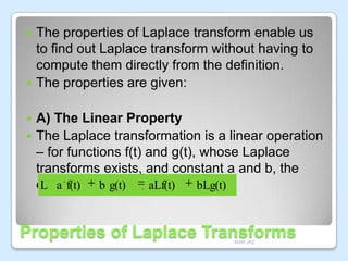
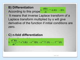
This document discusses Laplace transforms and their applications in control systems. It begins by defining the Laplace transform and explaining how it can be used to solve differential equations by transforming them from the time domain to the complex frequency domain. It then provides several properties and formulas for Laplace transforms, including derivatives, integrals, time shifts, and partial fraction decomposition. Examples are given to demonstrate finding the Laplace transform of common functions and taking the inverse Laplace transform. The document concludes by explaining how Laplace transforms can be used to analyze control systems modeled by integrodifferential equations.

1. CHAPTER 2
LAPLACE TRANSFORM
AND TRANSFER FUNCTION
MAR JKE

2. 




2.1 Explain the concept of Laplace Transform
2.2 Understand the concept of transfer function
2.3 Understand block diagram representation
2.4 Explain Signal Flow Graph representation
Identify the Mason’s gain formula
LAPLACE TRANSFORM AND TRANSFER
FUNCTION
MAR JKE

3. 
The transform method is used to solve certain
problems, that are difficult to solve directly.

In this method the original problems is first
transformed and solved.

Laplace transform is one of the tools for solving
ordinary linear differential equations.
Definition of Laplace Transform
MAR JKE

4. 
First : Convert the given differential equation
from time domain to complex frequency domain
by taking Laplace transform of the equation

From this equation, determine the Laplace
transform of the unknown variable

Finally, convert this expression into time domain
by taking inverse Laplace transform
MAR JKE

5. 
Laplace transform method of solving differential
equations offers two distinct advantages over
classical method of problem solving

From this equation, determine the Laplace
transform of the unknown variable

Finally, convert this expression into time domain
by taking inverse Laplace transform
MAR JKE

6. 
The Laplace transform is defined as below:
Let f(t) be a real function of a real variable t
defined for t>0, then f (t) .e dt
F(s) L f(t)
- st
0
Where F(s) is called Laplace transform of f(t).
And the variable ‘s’ which appears in F(s) is
frequency dependent complex variable
 It is given by, s σ jω
where
= Real part of complex variable ‘s’
= Imaginary part of complex
variable ‘s’

MAR JKE

7. Example 1

Find the Laplace transform of e-at and 1 for t ≥ 0
MAR JKE

8. 
Find the Laplace transform of e-at and 1 for t ≥ 0

Solution : i) f(t) = e-at

ii) f(t) = 1
MAR JKE

9. 
The operation of finding out time domain
function f(t) from Laplace transform F(s) is
called inverse Laplace transform and denoted
as L-1
-1
L F(s)
-1
L
L (f(t))
f(t)

Thus,

The time function f(t) and its Laplace transform
F(s) is called transform pair
Inverse Laplace Transform
MAR JKE

10. The properties of Laplace transform enable us
to find out Laplace transform without having to
compute them directly from the definition.
 The properties are given:

A) The Linear Property
 The Laplace transformation is a linear operation
– for functions f(t) and g(t), whose Laplace
transforms exists, and constant a and b, the
equation isb:g(t)
L a f(t)
aLf(t)
bLg(t)

Properties of Laplace Transforms
MAR JKE

11. B) Differentiation
df(t)
L
sLf(t) - f(0)
 According to this property, dt
 It means that inverse Laplace transform of a
Laplace transform multiplied by s will give
derivative of the function if initial conditions are
zero.

C) n-fold differentiation
n
 According to this property,
d f(t)

n
L
dt
n
s Lf(t) - s
n -1
f(0) - s
n -2
'
f (0) - ... f
n -1
MAR JKE
(0)

12. 
D) Integration Property
t
L
1
f ( )
s
In general, the Laplace transform of an order n
is
L
1
s

Lf(t)
s
0

1
f (0 )
n
....
Lf(t)
f(t)dt
f
n -1
s
n
(0)
n
f
n -2
s
(0)
n -1
n
...
f (0)
s
Laplace transform exists if f(t) does not grow too
t
fast as
MAR JKE

13. 
E) Time Shift

The Laplace transform of f(t) delayed by time T
is equal to the Laplace transform of f(t)
multiplied by e-sT ; that is
L[f ( t – T ) u( t – T )] = e-sT F(s), where u (t – T)
denotes the unit step function, which is shifted
to the right in time by T.
MAR JKE

14. F) Convolution Integral
 The Laplace transform of the product of two
functions F1(s) and F2(s) is given by the
convolution integrals
t

L
-1
F1 ( s)F 2 ( s)
f 1 ( t) f 2 ( t - )d
0
t
f 1 (t - )f 2 ( ) d
0
where L-1F1(s) = f1(t) and L-1F2(s) = f2(t)
MAR JKE

15. 
G) Product Transformation

The Laplace transform of the product of two
functions f1(t) and f2(t) is given by the complex
convolution integral
1
c
L
-1
f 1 ( t)f
2
j
( t)
2
j
F1 (
)F2 (
)d
c- j

H) Frequency Scaling

Thes inverse Laplace transform of the functions
F
af(at), where
-1
L F(s)
f(t)
a
MAR JKE

16. 
I) Time Scaling
 The
L f
Laplace transform of a functions
t
aF(as)
where
F(s)
Lf(t)
a
MAR JKE

17. J) Complex Translation
 If F(s) is the Laplace transform of f(t) then by the
complex translation property,

MAR JKE

18. 
K) Initial Value Theorem

The Laplace transform is very useful to find the
initial value of the time function f(t). Thus if F(s)
is the Laplace transform of f(t) then,

The only restriction is that f(t) must be
continuous or at the most , a step discontinuity
at t=0.
MAR JKE

19. 
L) Final Value Theorem

Similar to the initial value, the Laplace transform is
also useful to find the final value of the time function
f(t).
Thus if F(s) is the Laplace transform of f(t) then the
final value theorem states that,


The only restriction is that the roots of the
denominator polynomial of F(s) i.e poles of F(s)
have negative or zero real parts
MAR JKE

20. Example 2

Find the Laplace transform of sin t
MAR JKE

21. 
Find the Laplace transform of sin t
MAR JKE

22. MAR JKE

23. f(t)
F(s)
1
1/s
Constant K
K/s
K f(t), K is constant
K F(s)
t
1/s2
tn
n /sn+1
e-at
1/s+a
eat
1/s-a
e-at tn
n /((s+a)n+1 )
sin t
/(s2 +
2)
cos t
s/(s2 +
2)
e-at sin t
/((s+a)2 +
2)
Table of Laplace Transforms:
Table 1 : Standard Laplace Transform
pairs
MAR JKE

24. f(t)
e-at cos t
F(s)
(s+a)/((s+a)2 +
sinh t
/(s2 -
2)
cosh t
s/(s2 -
2)
t e-at
1/(s+a)2
1 - e-at
a/s(s+a)
Table 1 Contd….
MAR JKE
2)

25. Function f(t)
Laplace Transform F(s)
Unit step = u(t)
1/s
A u(t)
A/s
Delayed unit step = u(t-T)
e-Ts/s
A u(t-T)
Ae-Ts /s
Unit ramp = r(t) = t u(t)
1/s2
At u(t)
A/s2
Delayed unit ramp = r(t-T) = (t-T) u(tT)
e-Ts /s2
A(t-T) u(t-T)
Ae-Ts /s 2
Unit impulse = (t)
1
Delayed unit impulse = (t-T)
e-Ts
Impulse of strength K i.e K (t)
K
Table 2 : Laplace transforms of standard
time functions
MAR JKE

26. 
Let F(s) is the Laplace transform of f(t) then the
inverse Laplace transform is denoted as,
f(t)

-1
L
F(s)
The F(s), in partial fraction method, is written in the
form as,
F(s)
N(s)
D(s)


Where
N(s) = Numerator polynomial in s
D(s) = Denominator polynomial in s
Inverse Laplace Transform
MAR JKE

27. The roots of D(s) are simple and real
 The function F(s) can be expressed as,

N(s)
N(s)
D(s)
F(s)
(s - a)(s - b)(s - c)...
where a, b, c… are the simple and real roots
of D(s).

The degree of N(s) should be always less than
D(s)
Simple and Real Roots
MAR JKE

28. 
This can be further expressed as,
N(s)
K1
K2
K3
(s - a)(s - b)(s - c)...
F(s)
(s - a)
(s - b)
(s - c)
....
where K1, K2, K3 … are called partial fraction
coefficients
 The values of K1, K2, K3 … can be obtained as,
K1
(s - a). F(s)
K
(s - b). F(s)
2
K3
(s - c). F(s)
s
s
s
a
b
c
MAR JKE

29. 
In general,
K

Where sn = nth root of D(s)

n
L e
(s - s n ). F(s)
at
s
and so on
sn
1
(s  a)
Is standard Laplace transform pair.
 Once F(s) is expressed in terms of partial
fractions, with coefficients K1, K2 … Kn, the
inverse Laplace transform can be easily
obtained -1
at
bt
ct

f(t)
L F(s)
K 1e
K 2e
K 3e
MAR JKE
...

30. Example 3

Find the inverse Laplace transform of given F(s)
(s
F(s)
s(s
2)
3)(s
4)
MAR JKE

31. 
Solution : The degree of N(s) is less than D(s).
Hence F(s) can be expressed as,
F(s)
K1
s
where
(s
K1
K2
K3
1
F(s)
K3
K2
6
s
3)
s. F(s)
(s
(s
(s
s
0
3). F(s)
4). F(s)
4)
(s
s.
s(s
s
s
3
4
2)
3)(s
(s
2
4)
0
(s
3).
s(s
(s
s
s(s
3x4
6
2)
3)(s
(s
4 ).
1
(-3
4)
s
3
(-3)x(-3
2)
3)(s
(-4
4)
s
4
2)
(-4)x(-4
1
1
3 2
(s 3) ( s 4 )
MAR JKE
1
4)
2)
3
-
3)
1
2

32. 
Taking inverse Laplace transform,
f(t)
1
1
6
3
e
- 3t
-
1
e
- 4t
2
MAR JKE

33. 
The given function is of the form,
N(s)
F(s)
(s - a)
n
D(s)
There is multiple root of the order ‘n’ existing at
s=a.
 The method of writing the partial fraction
expansion for suchKmultiple roots K
is, N' (s)
K
K

F(s)
0
(s - a)
1
n
(s - a)
2
n -1
(s - a)
n -2
...
n -1
(s - a)
D' (s)
N' (s)
D' (s)
where
represents remaining terms of the
expansion of F(s)
Multiple Roots
MAR JKE

34. A separate coefficient is assumed for each
power of repetative root, starting from its highest
power n to 1
 For ease of solving simultaneous equations, find
the coefficient -K0 nby the same method for simple
K 0 (s a) . F(s) s a
roots


Finding the Laplace inverse transform of
expanded F(s) refer to standard transform pairs,
MAR JKE

35. Example 4

Obtain the inverse Laplace transform of given
f(s)
MAR JKE

36. MAR JKE

37. MAR JKE

38. MAR JKE

39. 
If there exists a quadratic term in D(s) of F(s) whose
roots are complex conjugates then the F(s) is
expressed with a first order polynomial in s in the
numerator as, As B
N' (s)
F(s)
(s
2
s
)
D' (s)

N' (s)
Where (s2 + s + ) is the quadratic whose roots
D' (s)
are complex conjugates while
represents
remaining terms of the expansion.

The A and B are partial fraction coefficients.
Complex Conjugate Roots
MAR JKE

40. The method of finding the coefficients is same
as the multiple roots.
 Once A and B are known, then use the following
method for calculating inverse Laplace
As B
transform.(s)
F
(s
s
)
 Consider
A and B are know.

1
2
2

Now complete the square in the denominator by
L.T.
4(F.T.)
calculating last term as,

Where L.T = Last term
term
F.T = First term
(M.T.)
M.T = Middle
MAR JKE

41. 2
L.T.
4
As
F1 ( s)
B
2
s
2
As
2
s
4
4
B
2
2
s
2
2
where
4

Now adjust the numerator As + B in such a way that
it is of the form
MAR JKE

42. Example 5

Find the inverse Laplace transform of
MAR JKE

43. MAR JKE

44. MAR JKE

45. MAR JKE

46. MAR JKE

47. MAR JKE

48. The control system can be classified as
electrical, mechanical, hydraulic, thermal and so
on.
 All system can be described by
integrodifferential equations of various orders
 While the o/p of such systems for any i/p can be
obtained by solving such integrodifferential
equations
 Mathematically, it is very difficult to solve such
equations in time domain

Application of Laplace Transform in
Control System
MAR JKE

49. 
The Laplace transform of such integrodifferential
equations converts them into simple algebraic
equations

All the complicated computations then can be
easily performed in s domain as the equations
to be handled are algebraic in nature.

Such transformed equations are known as
equations in frequency domain
MAR JKE

50. 
By eliminating unwanted variable, the required
variable in s domain can be obtained

By using technique of Laplace inverse, time
domain function for the required variable can be
obtained

Hence making the computations easy by
converting the integrodifferential equations into
algebraic is the main essence of the Laplace
transform
MAR JKE