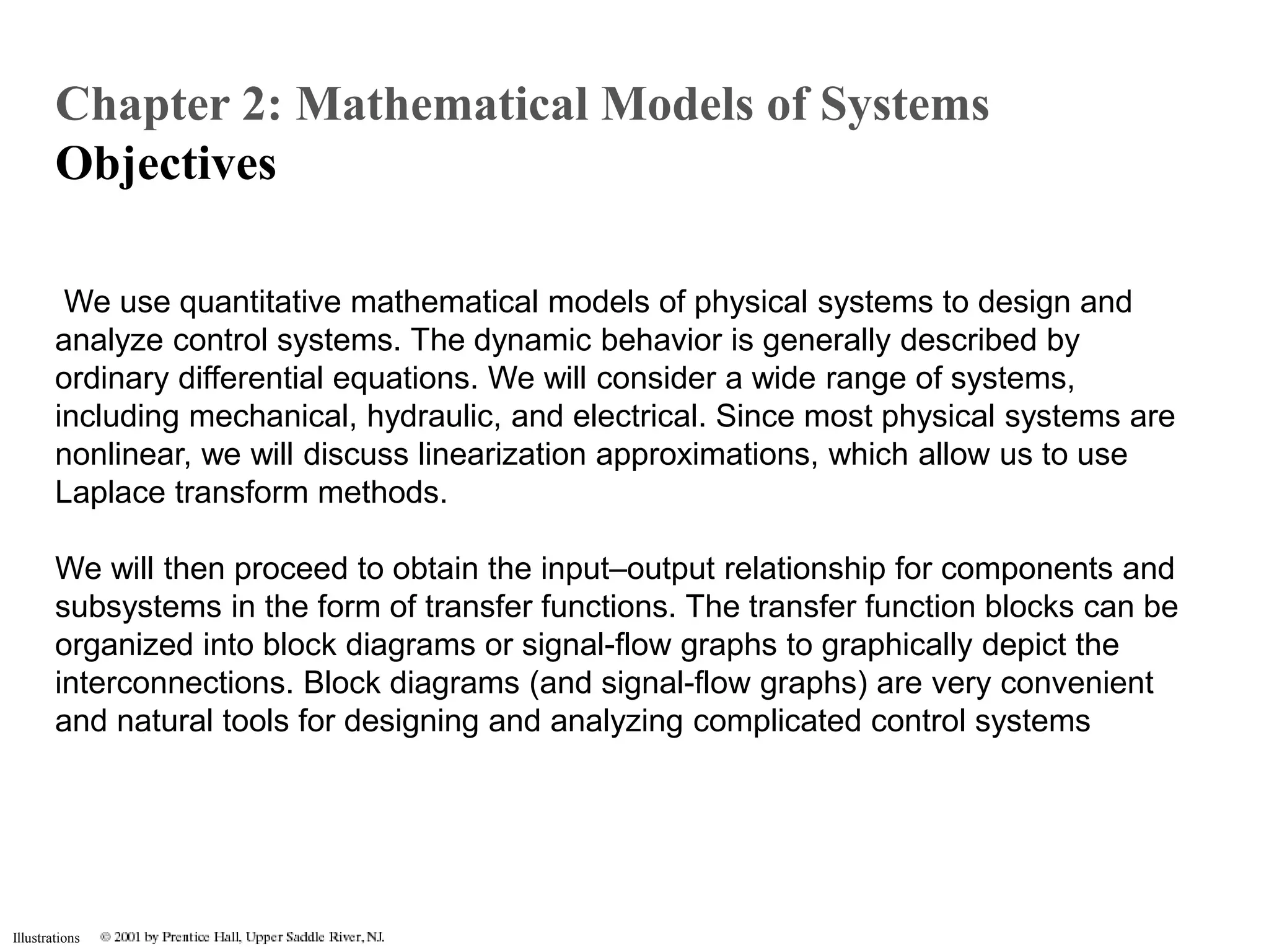
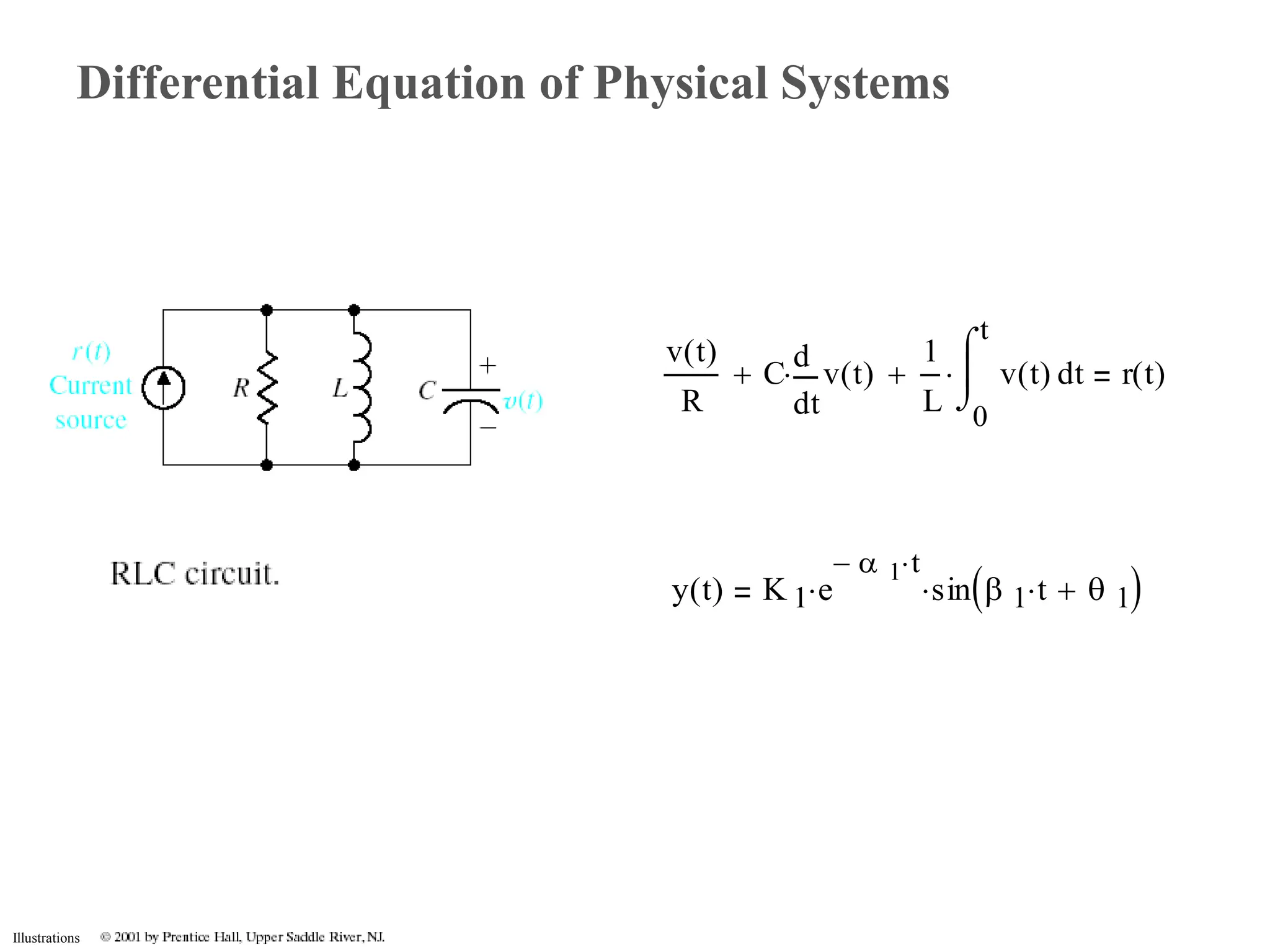
chapter-2.ppt control system slide for students

Illustrations
We use quantitative mathematical models of physical systems to design and
analyze control systems. The dynamic behavior is generally described by
ordinary differential equations. We will consider a wide range of systems,
including mechanical, hydraulic, and electrical. Since most physical systems are
nonlinear, we will discuss linearization approximations, which allow us to use
Laplace transform methods.
We will then proceed to obtain the input–output relationship for components and
subsystems in the form of transfer functions. The transfer function blocks can be
organized into block diagrams or signal-flow graphs to graphically depict the
interconnections. Block diagrams (and signal-flow graphs) are very convenient
and natural tools for designing and analyzing complicated control systems
Chapter 2: Mathematical Models of Systems
Objectives

Illustrations
Introduction
Six Step Approach to Dynamic System Problems
• Define the system and its components
• Formulate the mathematical model and list the necessary
assumptions
• Write the differential equations describing the model
• Solve the equations for the desired output variables
• Examine the solutions and the assumptions
• If necessary, reanalyze or redesign the system

Illustrations
Differential Equation of Physical Systems
Ta t
( ) Ts t
( )
 0
Ta t
( ) Ts t
( )
 t
( ) s t
( ) a t
( )

Ta t
( ) = through - variable
angular rate difference = across-variable

Illustrations
v21 L
t
i
d
d
 E
1
2
L
 i
2

v21
1
k t
F
d
d
 E
1
2
F
2
k

21
1
k t
T
d
d
 E
1
2
T
2
k

P21 I
t
Q
d
d
 E
1
2
I
 Q
2

Electrical Inductance
Translational Spring
Rotational Spring
Fluid Inertia
Describing Equation Energy or Power

Illustrations
Electrical Capacitance
Translational Mass
Rotational Mass
Fluid Capacitance
Thermal Capacitance
i C
t
v21
d
d
 E
1
2
M
 v21
2

F M
t
v2
d
d
 E
1
2
M
 v2
2

T J
t
2
d
d
 E
1
2
J
 2
2

Q Cf
t
P21
d
d
 E
1
2
Cf
 P21
2

q Ct
t
T2
d
d
 E Ct T2


Illustrations
Electrical Resistance
Translational Damper
Rotational Damper
Fluid Resistance
Thermal Resistance
F b v21
 P b v21
2

i
1
R
v21
 P
1
R
v21
2

T b 21
 P b 21
2

Q
1
Rf
P21
 P
1
Rf
P21
2

q
1
Rt
T21
 P
1
Rt
T21


Illustrations
M
2
t
y t
( )
d
d
2
 b
t
y t
( )
d
d

 k y t
( )

 r t
( )

Illustrations
v t
( )
R
C
t
v t
( )
d
d


1
L 0
t
t
v t
( )



d

 r t
( )
y t
( ) K 1 e
 1
 t

 sin  1 t
  1

 


Illustrations

Illustrations
K2 1
 2 .5
 2 10
 2 2

y t
( ) K2 e
2
 t

 sin 2 t
 2

 


y1 t
( ) K2 e
2
 t


 y2 t
( ) K2
 e
2
 t



0 1 2 3 4 5 6 7
1
0
1
y t
( )
y1 t
( )
y2 t
( )
t

Illustrations
Linear Approximations

Illustrations
Linear Approximations
Linear Systems - Necessary condition
Principle of Superposition
Property of Homogeneity
Taylor Series
http://www.maths.abdn.ac.uk/%7Eigc/tch/ma2001/notes/node46.html

Illustrations
Linear Approximations – Example 2.1
M 200gm
 g 9.8
m
s
2
 L 100cm
 0 0rad
  

15
 
16
 


T0 M g
 L
 sin 0
 


T1 
  M g
 L
 sin 
 


T2 
  M g
 L
 cos 0
 
  0

 
 T0


4 3 2 1 0 1 2 3 4
10
5
0
5
10
T1 
( )
T2 
( )

Students are encouraged to investigate linear approximation accuracy for different values of 0

Illustrations
The Laplace Transform
Historical Perspective - Heaviside’s Operators
Origin of Operational Calculus (1887)

Illustrations
p
t
d
d
1
p 0
t
u
1



d
i
v
Z p
( )
Z p
( ) R L p


i
1
R L p


H t
( )

1
L p 1
R
L p









H t
( )

1
R
R
L
1
p

R
L






2
1
p
2


R
L






3
1
p
3
 .....









 H t
( )

1
p
n
H t
( )

t
n
n
i
1
R
R
L
t

R
L






2
t
2
2

R
L






3
t
3
3

 ..














 i
1
R
1 e
R
L






 t









Expanded in a power series
v = H(t)
Historical Perspective - Heaviside’s Operators
Origin of Operational Calculus (1887)
(*) Oliver Heaviside: Sage in Solitude, Paul J. Nahin, IEEE Press 1987.

Illustrations
Definition
L f t
( )
( )
0

t
f t
( ) e
s
 t





d = F(s)
Here the complex frequency is s  j w


The Laplace Transform exists when
0

t
f t
( ) e
s
 t





d 

this means that the integral converges

Illustrations
Determine the Laplace transform for the functions
a) f1 t
( ) 1
 for t 0

F1 s
( )
0

t
e
s
 t




d

=
1
s
 e
s t

( )


1
s
b) f2 t
( ) e
a t

( )

F2 s
( )
0

t
e
a t

( )

e
s t

( )





d
=
1
s 1

 e
s a

( ) t

[ ]

 F2 s
( )
1
s a


Illustrations
note that the initial condition is included in the transformation
sF(s) - f(0+)
=
L
t
f t
( )
d
d







s
0

t
f t
( ) e
s t

( )





d

-f(0+) +
=
0

t
f t
( ) s
 e
s t

( )



 





d

f t
( ) e
s t

( )


=
0

v
u



d
we obtain
v f t
( )
and
du s
 e
s t

( )

 dt

and, from which
dv df t
( )
u e
s t

( )

where
u v
 u
v



d

=
v
u



d
by the use of
L
t
f t
( )
d
d






0

t
t
f t
( ) e
s t

( )


d
d




d
Evaluate the laplace transform of the derivative of a function

Illustrations
Practical Example - Consider the circuit.
The KVL equation is
4 i t
( )
 2
t
i t
( )
d
d

 0 assume i(0+) = 5 A
Applying the Laplace Transform, we have
0

t
4 i t
( )
 2
t
i t
( )
d
d








e
s t

( )






d 0 4
0

t
i t
( ) e
s t

( )





d
 2
0

t
t
i t
( ) e
s t

( )


d
d




d

 0
4 I s
( )
 2 s I s
( )
 i 0
( )

( )

 0 4 I s
( )
 2 s
 I s
( )

 10
 0
transforming back to the time domain, with our present knowledge of
Laplace transform, we may say that
I s
( )
5
s 2


0 1 2
0
2
4
6
i t
( )
t
t 0 0.01
 2

( )

i t
( ) 5 e
2 t

( )




Illustrations
The Partial-Fraction Expansion (or Heaviside expansion theorem)
Suppose that
The partial fraction expansion indicates that F(s) consists of
a sum of terms, each of which is a factor of the denominator.
The values of K1 and K2 are determined by combining the
individual fractions by means of the lowest common
denominator and comparing the resultant numerator
coefficients with those of the coefficients of the numerator
before separation in different terms.
F s
( )
s z1

s p1

( ) s p2

( )

or
F s
( )
K1
s p1

K2
s p2


Evaluation of Ki in the manner just described requires the simultaneous solution of n equations.
An alternative method is to multiply both sides of the equation by (s + pi) then setting s= - pi, the
right-hand side is zero except for Ki so that
Ki
s pi

( ) s z1

( )

s p1

( ) s p2

( )

s = - pi

Illustrations
s -> 0
t -> infinite
Lim s F s
( )

( )
Lim f t
( )
( )
7. Final-value Theorem
s -> infinite
t -> 0
Lim s F s
( )

( )
Lim f t
( )
( ) f 0
( )
6. Initial-value Theorem
0

s
F s
( )



d
f t
( )
t
5. Frequency Integration
F s a

( )
f t
( ) e
a t

( )


4. Frequency shifting
s
F s
( )
d
d

t f t
( )

3. Frequency differentiation
f at
( )
2. Time scaling
1
a
F
s
a







f t T

( ) u t T

( )

1. Time delay
e
s T

( )

F s
( )

Property Time Domain Frequency Domain

Illustrations
Useful Transform Pairs

Illustrations
y s
( )
s
b
M







yo
 

s
2 b
M






s


k
M







s 2 
 n


 
s
2
2 
 n

 n
2

s1  n

 
 n 
2
1



n
k
M

b
2 k M


 
s2  n

 
 n 
2
1



Roots
Real
Real repeated
Imaginary (conjugates)
Complex (conjugates)
s1  n

 
 j n
 1 
2



s2  n

 
 j n
 1 
2



Consider the mass-spring-damper system
Y s
( )
Ms b

( ) yo

Ms
2
bs
 k

equation 2.21

Illustrations

Illustrations
The Transfer Function of Linear Systems
V1 s
( ) R
1
Cs







I s
( )
 Z1 s
( ) R
Z2 s
( )
1
Cs
V2 s
( )
1
Cs






I s
( )

V2 s
( )
V1 s
( )
1
Cs
R
1
Cs

Z2 s
( )
Z1 s
( ) Z2 s
( )


Illustrations
Example 2.2
2
t
y t
( )
d
d
2
4
t
y t
( )
d
d

 3 y t
( )

 2 r t
( )

Initial Conditions: Y 0
( ) 1
t
y 0
( )
d
d
0 r t
( ) 1
The Laplace transform yields:
s
2
Y s
( )
 s y 0
( )


  4 s Y s
( )
 y 0
( )

( )

 3Y s
( )
 2 R s
( )

Since R(s)=1/s and y(0)=1, we obtain:
Y s
( )
s 4

( )
s
2
4s
 3

 
2
s s
2
4s
 3

 


The partial fraction expansion yields:
Y s
( )
3
2
s 1

( )
1

2
s 3

( )









1

s 1

( )
1
3
s 3

( )










2
3
s

Therefore the transient response is:
y t
( )
3
2
e
t


1
2
e
3
 t









1
 e
t
 1
3
e
3
 t









2
3

The steady-state response is:

t
y t
( )
lim

2
3

Illustrations

Illustrations
 Kf if

Tm K1 Kf
 if t
( )
 ia t
( )

field controled motor - Lapalce Transform
Tm s
( ) K1 Kf
 Ia

  If s
( )

Vf s
( ) Rf Lf s


  If s
( )

Tm s
( ) TL s
( ) Td s
( )

TL s
( ) J s
2
  s
( )
 b s
  s
( )


rearranging equations
TL s
( ) Tm s
( ) Td s
( )

Tm s
( ) Km If s
( )

If s
( )
Vf s
( )
Rf Lf s


Td s
( ) 0
 s
( )
Vf s
( )
Km
s J s
 b

( )
 Lf s
 Rf

 


Illustrations
V2 s
( )
V1 s
( )
1

RCs
V2 s
( )
V1 s
( )
RCs


Illustrations
V2 s
( )
V1 s
( )
R 2 R 1 C
 s
 1

 
R 1
V2 s
( )
V1 s
( )
R 1 C 1
 s
 1

 
 R 2 C 2
 s
 1

 
R 1 C 2
 s


Illustrations
 s
( )
Vf s
( )
K m
s J s
 b

( )
 Lf s
 R f

 
 s
( )
Va s
( )
K m
s R a La s


  J s
 b

( ) K b K m



 



Illustrations
Vo s
( )
Vc s
( )
K
Rc Rq







s c
 1

  s q
 1

 

c
Lc
Rc
q
Lq
Rq
For the unloaded case:
id 0 c q
0.05s c
 0.5s

V12 Vq V34 Vd
 s
( )
Vc s
( )
Km
s  s
 1

 

J
b m

( )
m = slope of linearized
torque-speed curve
(normally negative)

Illustrations
Y s
( )
X s
( )
K
s Ms B

( )
K
A kx

kp
B b
A
2
kp







kx
x
g
d
d
kp
P
g
d
d
g g x P

( ) flow
A = area of piston
Gear Ratio = n = N1/N2
N2 L
 N1 m

L n m

L n m


Illustrations
V2 s
( )
V1 s
( )
R2
R
R2
R1 R2

R2
R

max
V2 s
( ) ks 1 s
( ) 2 s
( )

 
V2 s
( ) ks error s
( )

ks
Vbattery
max

Illustrations
V2 s
( ) Kt  s
( )
 Kt s
  s
( )

Kt constant
V2 s
( )
V1 s
( )
ka
s 
 1

Ro = output resistance
Co = output capacitance
 Ro Co
  1s

and is often negligible
for controller amplifier

Illustrations
T s
( )
q s
( )
1
Ct s
 Q S

1
R








T To Te
 = temperature difference due to thermal process
Ct = thermal capacitance
= fluid flow rate = constant
= specific heat of water
= thermal resistance of insulation
= rate of heat flow of heating element
Q
S
Rt
q s
( )
xo t
( ) y t
( ) xin t
( )

Xo s
( )
Xin s
( )
s
2

s
2 b
M






s


k
M

For low frequency oscillations, where  n

Xo j 

 
Xin j 

 

2
k
M

Illustrations
x r 

converts radial motion to linear motion

Illustrations
Block Diagram Models

Illustrations
Original Diagram Equivalent Diagram
Original Diagram Equivalent Diagram

Illustrations
Example 2.7

Illustrations
Block Diagram Models Example 2.7

Illustrations
Signal-Flow Graph Models
For complex systems, the block diagram method can become
difficult to complete. By using the signal-flow graph model, the
reduction procedure (used in the block diagram method) is not
necessary to determine the relationship between system variables.

Illustrations
Y1 s
( ) G11 s
( ) R1 s
( )
 G12 s
( ) R2 s
( )


Y2 s
( ) G21 s
( ) R1 s
( )
 G22 s
( ) R2 s
( )



Illustrations
a11 x1
 a12 x2

 r1
 x1
a21 x1
 a22 x2

 r2
 x2

Illustrations
Example 2.8
Y s
( )
R s
( )
G1 G2
 G3
 G4
 1 L3
 L4

 


 
 G5 G6
 G7
 G8
 1 L1
 L2

 


 


1 L1
 L2
 L3
 L4
 L1 L3

 L1 L4

 L2 L3

 L2 L4



Illustrations
Example 2.10
Y s
( )
R s
( )
G1 G2
 G3
 G4

1 G2 G3
 H 2

 G3 G4
 H 1

 G1 G2
 G3
 G4
 H 3



Illustrations
Y s
( )
R s
( )
P1 P2 2

 P3


P1 G1 G2
 G3
 G4
 G5
 G6
 P2 G1 G2
 G7
 G6
 P3 G1 G2
 G3
 G4
 G8

 1 L1 L2
 L3
 L4
 L5
 L6
 L7
 L8

 
 L5 L7
 L5 L4

 L3 L4


 

1 3 1 2 1 L5
 1 G4 H4



Illustrations
Speed control of an electric traction motor.
Design Examples

Illustrations
The Simulation of Systems Using MATLAB

Illustrations
error
Sys1 = sysh2 / sysg4

Illustrations
error
Num4=[0.1];

Illustrations
Sequential Design Example: Disk Drive Read System

Illustrations
=
Sequential Design Example: Disk Drive Read System

Illustrations
1
L c s
 R c

Vc
Ic
K1
1
L q s
 R q

Vq
K2
K3
-Vb
+Vd
Km
Id
1
Ld La

  s
 R d R a

 

Tm
1
J s
 b

1
s

P2.11

Illustrations
http://www.jhu.edu/%7Esignals/sensitivity/index.htm

Illustrations
http://www.jhu.edu/%7Esignals/

chapter-2.ppt control system slide for students

More Related Content

Similar to chapter-2.ppt control system slide for students

Recently uploaded

chapter-2.ppt control system slide for students