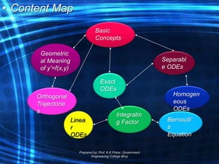
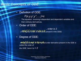
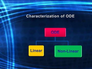
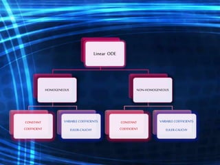
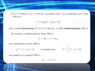
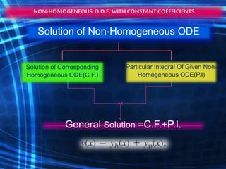
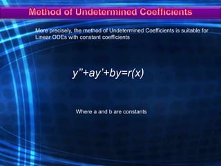
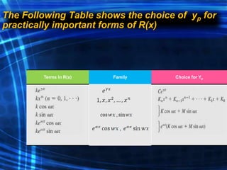
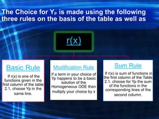
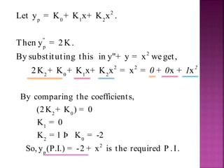
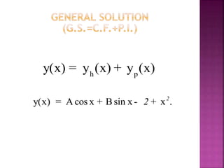
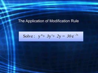
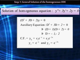
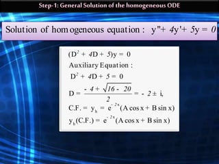
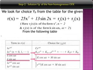
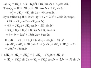
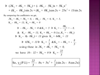
The document is a course outline for an advanced engineering mathematics class focused on ordinary differential equations (ODEs), detailing essential topics such as basic concepts, modeling, and types of first-order ODEs. It covers techniques for solving both homogeneous and non-homogeneous ODEs, including specific methods like variation of parameters and undetermined coefficients. The content serves as a resource for understanding mathematical modeling of physical phenomena in engineering.

1. ODE-
Ordinary Differential Equations
Advanced Engineering Mathematics
Course Code: 2130002
Gujarat Technological University
Prepared by: Prof. K.K.Pokar, Government Engineering College Bhuj

2. Rationale:
Differential equations are of basic
importance in engineering mathematics
because many physical laws and relations
appear mathematically in the form of a
differential equation.
Prepared by: Prof. K.K.Pokar, Government
Engineering College Bhuj

3. Content:
• Basic Concepts, Modeling
• Geometric Meaning of y’=f(x,y).
• Separable ODEs. Modeling
• Homogeneous ODEs
• Exact ODEs, Integrating Factors
• Linear ODEs, Bernoulli’s Equation &
Population Dynamics
• Orthogonal Trajectories
Prepared by: Prof. K.K.Pokar, Government
Engineering College Bhuj

4. • Content Map
Prepared by: Prof. K.K.Pokar, Government
Engineering College Bhuj
Basic
Concepts
Geometric
al Meaning
of y’=f(x,y)
Separabl
e ODEs
Exact
ODEs
Linea
r
ODEs
Integratin
g Factor Bernoulli’
s
Equation
Orthogonal
Trajectorie
s
Homogen
eous
ODEs

5. Basic Concepts of ODE
• Definition of ODE:
F(x,y,y’,y’’,….)=c
The equation involving independent and dependent variables and
their ordinary derrivatives.
• Order of ODE:
, order is 2
(The highest order of derivative present in the ODE)
• Degree of ODE:
the highest power of the highest order derivative present in the ODE is
called the order of
the ODE, here it is = 2
Prepared by: Prof. K.K.Pokar, Government
Engineering College Bhuj

6. Falling Stone from Leaning Tow
Prepared by: Prof. K.K.Pokar, Government
Engineering College Bhuj
y

7. Parachutist
Prepared by: Prof. K.K.Pokar, Government
Engineering College Bhuj
Velocity
v

8. Outflowing wate
Prepared by: Prof. K.K.Pokar, Government
Engineering College Bhuj
Under the influence of gravity the outflowing water has velocity

9. Vibrating mass on a spring
Prepared by: Prof. K.K.Pokar, Government
Engineering College Bhuj
m
y

10. Current I in RLC circuit
Prepared by: Prof. K.K.Pokar, Government
Engineering College Bhuj

11. Euler-Bernoulli beam theory
Prepared by: Prof. K.K.Pokar, Government
Engineering College Bhuj

12. Pendulum
Prepared by: Prof. K.K.Pokar, Government
Engineering College Bhuj

13. Lotka-Volterra predator-prey model
Prepared by: Prof. K.K.Pokar, Government
Engineering College Bhuj
Predator
Prey

14. Radio Active
Decay
Prepared by: Prof. K.K.Pokar, Government
Engineering College Bhuj

15. Types of first order ODEs

16. First Order
ODE
Separable
Reducible to
Separable
Homogeneous ODE
Non-Homogeneous
Reducible to
Homogeneous
Not Reducible
to Separable

17. Separable ODEs

19. Non Separable but Reducible to
Separable
Reducible to
Separable
Homogeneous
Reducible to
Homogeneous

20. Homogeneous ODE
• y’=f(x,y) is said to be homogeneous if f(x,y) is homogeneous.
OR
• Mdx + Ndy = 0 is said to be homogeneous if M(x,y) and N(x,y)
are both homogeneous functions of the same degree.
e.g., x dx + y dy = 0 ( homogeneous)
xy dx + y dy = 0 (non homogeneous)

21. Solving homogeneous ODE
• Take substitution y = vx
• y’ = v+xv’
• Substitute the above things into the given ODE
• That reduces it into the separable ODE in v and x.
• Solve it for v.
• Back substitute v=y/x.

22. Reducible to Homogeneous ODE
Zero
Non
zero

24. Linear ODE
HOMOGENEOUS
CONSTANT
COEFFICIENT
VARIABLE COEFFICIENTS
EULER-CAUCHY
NON-HOMOGENEOUS
CONSTANT
COEFFICIENT
VARIABLE COEFFICIENTS
EULER-CAUCHY

26. it

27. NON-HOMOGENEOUS O.D.E. WITHCONSTANTCOEFFICIENTS
Solution of Non-Homogeneous ODE
Solution of Corresponding
Homogeneous ODE(C.F.)
Particular Integral Of Given Non-
Homogeneous ODE(P.I)
General Solution =C.F.+P.I.

28. 1
F(D)

29. More precisely, the method of Undetermined Coefficients is suitable for
Linear ODEs with constant coefficients
y’’+ay’+by=r(x)
Where a and b are constants

30. The Following Table shows the choice of yp for
practically important forms of R(x)
Terms in R(x) Family Choice for Yp

31. The Choice for Yp is made using the following
three rules on the basis of the table as well as
r(x)
Basic Rule
If r(x) is one of the
functions given in the
first column of the table
2.1, choose Yp in the
same line.
Modification Rule
If a term in your choice of
Yp happens to be a basic
solution of the
Homogeneous ODE then
multiply your choice by x
Sum Rule
If r(x) is sum of functions in
the first column of the Table
2.1, choose for Yp the sum
of the functions in the
corresponding lines of the
second column.

32. The Application of Basic Rule
Solve
2
y'' + y = x

33. 2
2
0x
h
h
(D + 1)y = 0
Auxiliary Equation :D + 1 = 0
D = ± i
C.F. y = e (A cos x + B sin x)
y (C.F.) = A cos x + B sin x
=

34. We look for choice Yp from the table for the given
2 n
r(x) = x (Of theform x ,n )= 2
From the following table

35. 2
p 0 1 2
''
p
2
2 2
2 0 1 2
Let y = K + K x+ K x .
Then y = 2K.
By substituting this in y''+ y = x weget,
2K + K + K x+ K x = x x x= + + 2
0 0 1
2 0
1
2 0
2
p
By comparing the coefficients,
(2K + K ) = 0
K = 0
K = 1 K = -2
So, y (P.I.) = -2 + x is the required P .I.
Þ

36. y(x) A cos x B sin x x .= + - + 2
2
h p
y(x) y (x) y (x)= +

37. The Application of Modification Rule
x
Solve : y '' y ' y e-
+ + = 2
3 2 30

38. 2
2
x x
h
x x
(D + D )y = 0
Auxiliary Equation :D + D = 0
(D )(D )
D ,
C.F. y = c e c e
y e and y e
- -
- -
+
+
Þ + + =
Þ = - -
= +
= =
2
1 2
2
1 2
3 2
3 2
1 2 0
1 2
Solution of homogeneous equation : y'' y' y+ + =3 2 0

39. We look for choice Yp from the table for the given
2x x
r(x) = e (Of theform Ke )-
30
From the following table

40. x
y e-
= 2
2
' x x
p
'' x x
p
'' ' x
p p p
x x x x x x
x x x x x x
Then y Ke Kxe
&y Ke Kxe
Substituting these values in in the given diff. eqn.
y y y e
Ke Kxe (Ke Kxe ) Kxe e
Ke Kxe Ke Kxe Kxe e
- -
- -
-
- - - - - -
- - - - - -
= -
= - +
+ + =
Þ - + + - + =
Þ - + + - + =
2 2
2 2
2
2 2 2 2 2 2
2 2 2 2 2 2
2
4 4
3 2 30
4 4 3 2 2 30
4 4 3 6 2 30
x x
x
p
Ke e
By comparing the coefficien t
K
y (P.I.) = xe is the required P .I.
- -
-
Þ - =
= -
-
2 2
2
30
30
30
But if we look at the C.F. it has the solution
which is same as choice of
x
p
y Ke-
= 2
So, by modification rule we have to multiply the above choice of Yp
by x, i.e., we have the modified choice
x
p
y Kxe-
= 2

41. x x x
y(x) c e c e xe .- - -
= + -2 2
1 2
30
h p
y(x) y (x) y (x)= +

42. r(x) Sum Rule
The Application of Sum Rule
Solve : y '' y ' y x sin x+ + = +2
4 5 25 13 2

43. x
h
x
h
(D D )y = 0
Auxiliary Equation :
D D = 0
D i,
C.F. y = e (A cos x + B sin x)
y (C.F.) = e (A cos x + B sin x)
-
-
+ +
+ +
- + -
= = - ±
=
2
2
2
2
4 5
4 5
4 16 20
2
2
Solution of homogeneous equation : y'' y' y+ + =4 5 0

44. Step-2: Solution Yp of the Non-homogeneous ODE
We look for choice Yp from the table for the given
r(x) = x sin x r (x) r (x)+ = +2
1 2
25 13 2
From the following table
n
( Here r (x) is of the form x , n
& r (x) is of the form k sin x, ) 
=
=
1
2
2
2
.

45. 2
p 0 1 2
'
p
''
p
Let y = (K + K x+ K x ) (K sin x K cos x).
Then y = K K x K cos x K sin x.
y = K K sin x K cos x.
+ +
+ + -
- -
3 4
1 2 3 4
2 3 4
2 2
2 2 2 2 2
2 4 2 4 2
2
2
0 1 2
By substituting this in y''+ y ' y = x sin x, weget,
( K K sin x K cos x)
(K K x K cos x K sin x)
(K + K x+ K x K sin x K cos x)
x x sin x cos x
+ +
- -
+ + + -
+ + +
= + + + +
2 3 4
1 2 3 4
3 4
2
4 5 25 13 2
2 4 2 4 2
4 2 2 2 2 2
5 2 2
0 0 25 13 2 0 2
( K K K ) ( K K )x K x
( K K K )sin x ( K K K )cos x
x sin x
Þ + + + - - +
+ - - + + - + +
= +
2
2 1 0 2 1 2
3 4 3 4 3 4
2
2 4 5 8 5 5
4 8 5 2 4 8 5 2
25 13 2
( K K K ) ( K K )x K x
(K K ) sin x (K K ) cos x x sin x
Þ + + + - - +
+ - + + = +
2
2 1 0 2 1 2
2
3 4 4 3
2 4 5 8 5 5
8 2 8 2 25 13 2

46. ( K K K ) ( K K )x K x
(K K ) sin x (K K ) cos x x sin x
Þ + + + - - +
+ - + + = +
2
2 1 0 2 1 2
2
3 4 4 3
2 4 5 8 5 5
8 2 8 2 25 13 2
By comparing the coefficients we get,
K K K , K K , K ,
K K , K K
+ + = - - = =
- = + =
2 1 0 2 1 2
3 4 4 3
2 4 5 0 8 5 0 5
8 13 8 0
K
K K &K K .
& K K , K K ( i.e.,K K )
Þ - - = = Þ = - = -
- = + = = -
2
2 1 2 1
3 4 4 3 4 3
8
8 5 0 5 8
5
8 13 8 0 8
K ( K ) gives K K
K K &K K .
u sin g these in K K K ,
we have K K
Þ - - = + =
Þ = Þ = = - = -
+ + =
- + = Þ =
3 3 3 3
3 3 4 3
2 1 0
0 0
8 8 13 64 13
1 8
65 13 8
5 5
2 4 5 0
22
10 32 5 0
5
p
So, y (P.I.) x x (sin x cos x)= - + + -222 1
8 5 2 8 2
5 5

47. x
y(x) e (A cos x + B sin x) x x (sin x cos x).
-
= + - + + -
2 222 1
8 5 2 8 2
5 5
h p
y(x) y (x) y (x)= +

48. 421
0011 0010 1010 1101 0001 0100 1011 Method of
Finding Particular
Integral
Method of
Variation of
Parameters

49. 421
0011 0010 1010 1101 0001 0100 1011
Method of Variation of Parameters

50. 421
0011 0010 1010 1101 0001 0100 1011
x
h
h
(D )y = 0
Auxiliary Equation :D = 0 D i,
C.F. y = e (A cos x + B sin x)
y (C.F.) = A cos x + B sin x
Next, we find theP.I.
Here we have y cos x and y sin x
+
+ Þ = ±
=
= =
2
2
0
1 2
1
1
Solution of homogeneous equation : y'' y+ = 0
' '
So,W W(y ,y ) y y y y
cosx(cosx) sin x( sin x) cos x sin x
= = -
= - - = +
=
1 2 1 2 2 1
2 2
1
Method of Variation of Parameters

51. 421
0011 0010 1010 1101 0001 0100 1011
Next, we have the formula,
General solution is

52. Method of variation of
parameres for higher order ODE

53. Variation of Parameters: Nonhomogeneous
Euler-Cauchy Equation
Solution:
D’(D’ – 1)(D’ – 2) – 3 D’(D’ – 1) + 6D’ – 6 =0
D’=1, 2, 3
C.F.= c1 x + c2 x2 + c3 x3

54. Step-2:
Evaluation of Wronskian

55. Step -3: Evaluation of P.I.