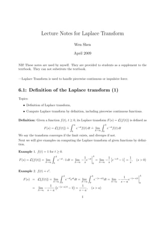
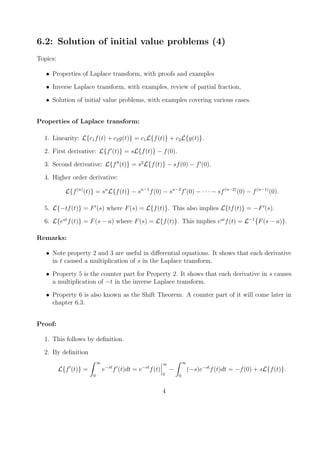
- The document provides lecture notes on the Laplace transform, including definitions, properties, examples of computing Laplace transforms, and using Laplace transforms to solve initial value problems. - The key aspects covered are the definition of the Laplace transform, examples of computing Laplace transforms of various functions, properties of the Laplace transform including how derivatives relate to the transform, and using Laplace transforms to solve initial value problems by taking the transform of both sides, solving for the transformed function Y(s), and then taking the inverse transform. - Solutions of initial value problems using Laplace transforms generally involve taking the transform of both sides, solving the resulting algebraic equation for Y(s), and then taking the inverse Laplace transform of Y(s) to find the

1. Lecture Notes for Laplace Transform
Wen Shen
April 2009
NB! These notes are used by myself. They are provided to students as a supplement to the
textbook. They can not substitute the textbook.
—Laplace Transform is used to handle piecewise continuous or impulsive force.
6.1: Definition of the Laplace transform (1)
Topics:
• Definition of Laplace transform,
• Compute Laplace transform by definition, including piecewise continuous functions.
Definition: Given a function f(t), t ≥ 0, its Laplace transform F(s) = L{f(t)} is defined as
F(s) = L{f(t)}
.
=
Z ∞
0
e−st
f(t) dt
.
= lim
A→∞
Z A
0
e−st
f(t) dt
We say the transform converges if the limit exists, and diverges if not.
Next we will give examples on computing the Laplace transform of given functions by defini-
tion.
Example 1. f(t) = 1 for t ≥ 0.
F(s) = L{f(t)} = lim
A→∞
Z A
0
e−st
· 1 dt = lim
A→∞
−
1
s
e−st
¯
¯
¯
¯
A
0
= lim
A→∞
−
1
s
£
e−sA
− 1
¤
=
1
s
, (s > 0)
Example 2. f(t) = et
.
F(s) = L{f(t)} = lim
A→∞
Z A
0
e−st
eat
dt = lim
A→∞
Z A
0
e−(s−a)t
dt = lim
A→∞
−
1
s − a
e−(s−a)t
¯
¯
¯
¯
A
0
= lim
A→∞
−
1
s − a
¡
e−(s−a)A
− 1
¢
=
1
s − a
, (s > a)
1

2. Example 3. f(t) = tn
, for n ≥ 1 integer.
F(s) = lim
A→∞
Z A
0
e−st
tn
dt = lim
A→∞
(
tn e−st
−s
¯
¯
¯
¯
A
0
−
Z A
0
ntn−1
e−st
−s
dt
)
= 0 +
n
s
lim
A→∞
Z A
0
e−st
tn−1
dt =
n
s
L{tn−1
}.
So we get a recursive relation
L{tn
} =
n
s
L{tn−1
}, ∀n,
which means
L{tn−1
} =
n − 1
s
L{tn−2
}, L{tn−2
} =
n − 2
s
L{tn−3
}, · · ·
By induction, we get
L{tn
} =
n
s
L{tn−1
} =
n
s
(n − 1)
s
L{tn−2
} =
n
s
(n − 1)
s
(n − 2)
s
L{tn−3
}
= · · · =
n
s
(n − 1)
s
(n − 2)
s
· · ·
1
s
L{1} =
n!
sn
1
s
=
n!
sn+1
, (s > 0)
Example 4. Find the Laplace transform of sin at and cos at.
Method 1. Compute by definition, with integration-by-parts, twice. (lots of work...)
Method 2. Use the Euler’s formula
eiat
= cos at + i sin at, ⇒ L{eiat
} = L{cos at} + iL{sin at}.
By Example 2 we have
L{eiat
} =
1
s − ia
=
1(s + ia)
(s − ia)(s + ia)
=
s + ia
s2 + a2
=
s
s2 + a2
+ i
a
s2 + a2
.
Comparing the real and imaginary parts, we get
L{cos at} =
s
s2 + a2
, L{sin at} =
a
s2 + a2
, (s > 0).
Remark: Now we will use
R ∞
0
instead of limA→∞
R A
0
, without causing confusion.
For piecewise continuous functions, Laplace transform can be computed by integrating each
integral and add up at the end.
Example 5. Find the Laplace transform of
f(t) =
½
1, 0 ≤ t < 2,
t − 2, 2 ≤ t.
2

3. We do this by definition:
F(s) =
Z ∞
0
e−st
f(t) dt =
Z 2
0
e−st
dt +
Z ∞
2
(t − 2)e−st
dt
=
1
−s
e−st
¯
¯
¯
¯
2
t=0
+ (t − 2)
1
−s
e−st
¯
¯
¯
¯
∞
t=2
−
Z A
2
1
−s
e−st
dt
=
1
−s
(e−2s
− 1) + (0 − 0) +
1
s
1
−s
e−st
¯
¯
¯
¯
∞
t=2
=
1
−s
(e−2s
− 1) +
1
s2
e−2s
3

4. 6.2: Solution of initial value problems (4)
Topics:
• Properties of Laplace transform, with proofs and examples
• Inverse Laplace transform, with examples, review of partial fraction,
• Solution of initial value problems, with examples covering various cases.
Properties of Laplace transform:
1. Linearity: L{c1f(t) + c2g(t)} = c1L{f(t)} + c2L{g(t)}.
2. First derivative: L{f0
(t)} = sL{f(t)} − f(0).
3. Second derivative: L{f00
(t)} = s2
L{f(t)} − sf(0) − f0
(0).
4. Higher order derivative:
L{f(n)
(t)} = sn
L{f(t)} − sn−1
f(0) − sn−2
f0
(0) − · · · − sf(n−2)
(0) − f(n−1)
(0).
5. L{−tf(t)} = F0
(s) where F(s) = L{f(t)}. This also implies L{tf(t)} = −F0
(s).
6. L{eat
f(t)} = F(s − a) where F(s) = L{f(t)}. This implies eat
f(t) = L−1
{F(s − a)}.
Remarks:
• Note property 2 and 3 are useful in differential equations. It shows that each derivative
in t caused a multiplication of s in the Laplace transform.
• Property 5 is the counter part for Property 2. It shows that each derivative in s causes
a multiplication of −t in the inverse Laplace transform.
• Property 6 is also known as the Shift Theorem. A counter part of it will come later in
chapter 6.3.
Proof:
1. This follows by definition.
2. By definition
L{f0
(t)} =
Z ∞
0
e−st
f0
(t)dt = e−st
f(t)
¯
¯
¯
∞
0
−
Z ∞
0
(−s)e−st
f(t)dt = −f(0) + sL{f(t)}.
4

5. 3. This one follows from Property 2. Set f to be f0
we get
L{f00
(t)} = sL{f0
(t)}−f0
(0) = s(sL{f(t)}−f(0))−f0
(0) = s2
L{f(t)}−sf(0)−f0
(0).
4. This follows by induction, using property 2.
5. The proof follows from the definition:
F0
(s) =
d
ds
Z ∞
0
e−st
f(t)dt =
Z ∞
0
∂
∂s
(e−st
)f(t)dt =
Z ∞
0
(−t)e−st
f(t)dt = L{−tf(t)}.
6. This proof also follows from definition:
L{eat
f(t)}
Z ∞
0
e−st
eat
f(t)dt =
Z ∞
0
e−(s−a)t
f(t)dt = F(s − a).
By using these properties, we could find more easily Laplace transforms of many other func-
tions.
Example 1.
From L{tn
} =
n!
sn+1
, we get L{eat
tn
} =
n!
(s − a)n+1
.
Example 2.
From L{sin bt} =
b
s2 + b2
, we get L{eat
sin bt} =
b
(s − a)2 + b2
.
Example 3.
From L{cos bt} =
s
s2 + b2
, we get L{eat
cos bt} =
s − a
(s − a)2 + b2
.
Example 4.
L{t3
+ 5t − 2} = L{t3
} + 5L{t} − 2L{1} =
3!
s4
+ 5
1
s2
− 2
1
s
.
Example 5.
L{e2t
(t3
+ 5t − 2)} =
3!
(s − 2)4
+ 5
1
(s − 2)2
− 2
1
s − 2
.
5

6. Example 6.
L{(t2
+ 4)e2t
− e−t
cos t} =
2
(s − 2)3
+
4
s − 2
−
s + 1
(s + 1)2 + 1
,
because
L{t2
+ 4} =
2
s3
+
4
s
, ⇒ L{(t2
+ 4)e2t
} =
2
(s − 2)3
+
4
s − 2
.
Next are a few examples for Property 5.
Example 7.
Given L{eat
} =
1
s − a
, we get L{teat
} = −
µ
1
s − a
¶0
=
1
(s − a)2
Example 8.
L{t sin bt} = −
µ
b
s2 + b2
¶0
=
−2bs
(s2 + b2)2
.
Example 9.
L{t cos bt} = −
µ
s
s2 + b2
¶0
= · · · =
s2
− b2
(s2 + b2)2
.
6

7. Inverse Laplace transform. Definition:
L−1
{F(s)} = f(t), if F(s) = L{f(t)}.
Technique: find the way back.
Some simple examples:
Example 10.
L−1
½
3
s2 + 4
¾
= L−1
½
3
2
·
2
s2 + 22
¾
=
3
2
L−1
½
2
s2 + 22
¾
=
3
2
sin 2t.
Example 11.
L−1
½
2
(s + 5)4
¾
= L−1
½
1
3
·
6
(s + 5)4
¾
=
1
3
L−1
½
3!
(s + 5)4
¾
=
1
3
e−5t
L−1
½
3!
s4
¾
=
1
3
e−5t
t3
.
Example 12.
L−1
½
s + 1
s2 + 4
¾
= L−1
½
s
s2 + 4
¾
+
1
2
L−1
½
2
s2 + 4
¾
= cos 2t
1
2
sin 2t.
Example 13.
L−1
½
s + 1
s2 − 4
¾
= L−1
½
s + 1
(s − 2)(s + 2)
¾
= L−1
½
3/4
s − 2
+
1/4
s + 2
¾
=
3
4
e2t
+
1
4
e−2t
.
Here we used partial fraction to find out:
s + 1
(s − 2)(s + 2)
=
A
s − 2
+
B
s + 2
, A = 3/4, B = 1/4.
7

8. Solutions of initial value problems.
We will go through one example first.
Example 14. (Two distinct real roots.) Solve the initial value problem by Laplace transform,
y00
− 3y0
− 10y = 2, y(0) = 1, y0
(0) = 2.
Step 1. Take Laplace transform on both sides: Let L{y(t)} = Y (s), and then
L{y0
(t)} = sY (s) − y(0) = sY − 1, L{y00
(t)} = s2
Y (s) − sy(0) − y0
(0) = s2
Y − s − 2.
Note the initial conditions are the first thing to go in!
L{y00
(t)} − 3L{y0
(t)} − 10L{y(t)} = L{2}, ⇒ s2
Y − s − 2 − 3(sY − 1) − 10Y =
2
s
.
Now we get an algebraic equation for Y (s).
Step 2: Solve it for Y (s):
(s2
− 3s − 10)Y (s) =
2
s
+ s + 2 − 3 =
s2
− s + 2
s
, ⇒ Y (s) =
s2
− s + 2
s(s − 5)(s + 2)
.
Step 3: Take inverse Laplace transform to get y(t) = L−1
{Y (s)}. The main technique here is
partial fraction.
Y (s) =
s2
− s + 2
s(s − 5)(s + 2)
=
A
s
+
B
s − 5
+
C
s + 2
=
A(s − 5)(s + 2) + Bs(s + 2) + Cs(s − 5)
s(s − 5)(s + 2)
.
Compare the numerators:
s2
− s + 2 = A(s − 5)(s + 2) + Bs(s + 2) + Cs(s − 5).
The previous equation holds for all values of s.
Set s = 0: we get −10A = 2, so A = −1
5
.
Set s = 5: we get 35B = 22, so B = 22
35
.
Set s = −2: we get 14C = 8, so C = 4
7
.
Now, Y (s) is written into sum of terms which we can find the inverse transform:
y(t) = AL−1
{
1
s
} + BL−1
{
1
s − 5
} + CL−1
{
1
s + 2
} = −
1
5
+
22
35
e5t
+
4
7
e−2t
.
8

9. Structure of solutions:
• Take Laplace transform on both sides. You will get an algebraic equation for Y .
• Solve this equation to get Y (s).
• Take inverse transform to get y(t) = L−1
{y}.
Example 15. (Distinct real roots, but one matches the source term.) Solve the initial value
problem by Laplace transform,
y00
− y0
− 2y = e2t
, y(0) = 0, y0
(0) = 1.
Take Laplace transform on both sides of the equation, we get
L{y00
} − L{y0
} − L{2y} = L{e2t
}, ⇒ s2
Y (s) − 1 − sY (s) − 2Y (s) =
1
s − 2
.
Solve it for Y :
(s2
−s−2)Y (s) =
1
s − 2
+1 =
s − 1
s − 2
, ⇒ Y (s) =
s − 1
(s − 2)(s2 − s − 2)
=
s − 1
(s − 2)2(s + 1)
.
Use partial fraction:
s − 1
(s − 2)2(s + 1)
=
A
s + 1
+
B
s − 2
+
C
(s − 2)2
.
Compare the numerators:
s − 1 = A(s − 2)2
+ B(s + 1)(s − 2) + C(s + 1)
Set s = −1, we get A = −2
9
. Set s = 2, we get C = 1
3
. Set s = 0 (any convenient values of s
can be used in this step), we get B = 2
9
. So
Y (s) = −
2
9
1
s + 1
+
2
9
1
s − 2
+
1
3
1
(s − 2)2
and
y(t) = L−1
{Y } = −
2
9
e−t
+
2
9
e2t
+
1
3
te2t
.
Compare this to the method of undetermined coefficient: general solution of the equation
should be y = yH + Y , where yH is the general solution to the homogeneous equation and
Y is a particular solution. The characteristic equation is r2
− r − 2 = (r + 1)(r − 2) = 0,
so r1 = −1, r2 = 2, and yH = c1e−t
+ c2e2t
. Since 2 is a root, so the form of the particular
solution is Y = Ate2t
. This discussion concludes that the solution should be of the form
y = c1e−t
+ c2e2t
+ Ate2t
for some constants c1, c2, A. This fits well with our result.
9

10. Example 16. (Complex roots.)
y00
− 2y0
+ 2y = e−t
, y(0) = 0, y0
(0) = 1.
Before we solve it, let’s use the method of undetermined coefficients to find out which terms
will be in the solution.
r2
− 2r + 2 = 0, (r − 1)1
+ 1 = 0, r1,2 = 1 ± i,
yH = c1et
cos t + c2et
sin t, Y = Ae−t
,
so the solution should have the form:
y = yH + Y = c1et
cos t + c2et
sin t + Ae−t
.
The Laplace transform would be
Y (s) = c1
s − 1
(s − 1)2 + 1
+ c2
1
(s − 1)2 + 1
+ A
1
s + 1
=
c1(s − 1) + c2
(s − 1)2 + 1
+
A
s + 1
.
This gives us idea on which terms to look for in partial fraction.
Now let’s use the Laplace transform:
Y (s) = L{y}, L{y0
} = sY − y(0) = sY, L{y00
} = s2
Y − sy(0) − y(0) = s2
Y − 1.
s2
Y − 1 − 2sY + 2Y =
1
s + 1
, ⇒ (s2
− 2s + 2)Y (s) =
1
s + 1
+ 1 =
s + 2
s + 1
Y (s) =
s + 2
(s + 1)(s2 − 2s + 2)
=
s + 2
(s + 1)((s − 1)2 + 1)
=
A
s + 1
+
B(s − 1) + C
(s − 1)2 + 1
Compare the numerators:
s + 2 = A((s − 1)2
+ 1) + (B(s − 1) + C)(s + 1).
Set s = −1: 5A = 1, A = 1
5
.
Compare coefficients of s2
-term: A + B = 0, B = −A = −1
5
.
Set any value of s, say s = 0: 2 = 2A − B + C, C = 2 − 2A + B = 9
5
.
Y (s) =
1
5
1
s + 1
−
1
5
s − 1
(s − 1)2 + 1
+
9
5
1
(s − 1)2 + 1
y(t) =
1
5
e−t
−
1
5
et
cos t +
9
5
et
sin t.
We see this fits our prediction.
10

11. Example 17. (Pure imaginary roots.)
y00
+ y = cos 2t, y(0) = 2, y0
(0) = 1.
Again, let’s first predict the terms in the solution:
r2
+ 1 = 0, r1,2 = ±i, yH = c1 cos t + c2 sin t, Y = A cos 2t
so
y = yH + Y = c1 cos t + c2 sin t + A cos 2t,
and the Laplace transform would be
Y (s) = c1
s
s1 + 1
+ c2
1
s2 + 1
+ A
s
s2 + 4
.
Now, let’s take Laplace transform on both sides:
s2
Y − 2s − 1 + Y = L{cos 2t} =
s
s2 + 4
(s2
+ 1)Y (s) =
s
s2 + 4
+ 2s + 1 =
2s3
+ s2
+ 9s + 4
s2 + 4
Y (s) =
2s3
+ s2
+ 9s + 4
(s2 + 4)(s2 + 1)
=
As + B
s2 + 1
+
Cs + D
s2 + 4
.
Comparing numerators, we get
2s3
+ s2
+ 9s + 4 = (As + B)(s2
+ 4) + (Cs + D)(s2
+ 1).
One may expand the right-hand side and compare terms to find A, B, C, D, but that takes
more work. Let’s try by setting s into complex numbers.
Set s = i, and remember the facts i2
= −1 and i3
= −i, we have
−2i − 1 + 9i + 4 = (Ai + B)(−1 + 4), 3 + 7i = 3B + 3Ai, B = 1, A =
7
3
.
Set now s = 2i:
−16i − 4 + 18i + 4 = (2Ci + D)(−3), 0 + 2i = −3D − 6Ci, D = 0, C = −
1
3
.
So
Y (s) =
7
3
s
s2 + 1
+
1
s2 + 1
−
1
3
s
s2 + 4
and
y(t) =
7
3
cos t + sin t −
1
3
cos 2t.
11

12. A very brief review on partial fraction, targeted towards inverse Laplace trans-
form.
Goal: rewrite a fractional form Pn(s)
Pm(s)
(where Pn is a polynomial of degree n) into sum of
“simpler” terms. We assume n < m.
The type of terms appeared in the partial fraction is solely determined by the denominator
Pm(s). First, fact out Pm(s), write it into product of terms of (i) s − a, (ii) s2
+ a2
, (iii)
(sa)2
+ b2
. The following table gives the terms in the partial fraction and their corresponding
inverse Laplace transform.
term in PM (s) from where? term in partial fraction inverse L.T.
real root, or
s − a g(t) = eat A
s − a
Aeat
double roots,
(s − a)2
or r = a and g(t) = eat A
s − a
+
B
(s − a)2
Aeat
+ Bteat
double roots,
(s − a)3
and g(t) = eat A
s − a
+
B
(s − a)2
+
C
(s − a)3
Aeat
+ Bteat
+
C
2
t2
eat
imaginary roots or
s2
+ µ2
g(t) = cos µt or sin µt
As + B
s2 + µ2
A cos µt + B sin µt
complex roots, or
(s − λ)2
+ µ2
g(t) = eλt
cos µt(or sin µt)
A(s − λ) + B
(s − λ)2 + µ2
eλt
(A cos µt + B sin µt)
In summary, this table can be written
Pn(s)
(s − a)(s − b)2(s − c)3((s − λ)2 + µ2)
=
A
s − a
+
B1
s − b
+
B2
(s − b)2
+
C1
s − c
+
C2
(s − c)2
+
C3
(s − c)3
+
D1(s − λ) + D2
(s − λ)2 + µ2
.
12

13. 6.3: Step functions (2)
Topics:
• Definition and basic application of unit step (Heaviside) function,
• Laplace transform of step functions and functions involving step functions (piecewise
continuous functions),
• Inverse transform involving step functions.
We use steps functions to form piecewise continuous functions.
Unit step function(Heaviside function):
uct =
½
0, 0 ≤ t < c,
1, c ≤ t.
for c ≥ 0. A plot of uc(t) is below:
c
0
u
c
t
1
For a given function f(t), if it is multiplied with uc(t), then
uctf(t) =
½
0, 0 < t < c,
f(t), c ≤ t.
We say uc picks up the interval [c, ∞).
Example 1. Consider
1 − uc(t) =
½
1, 0 ≤ t < c,
0, c ≤ t.
A plot of this is given below
c
0
u
c
t
1
1−
13

14. We see that this function picks up the interval [0, c).
Example 2. Rectangular pulse. The plot of the function looks like
b
0
u
t
1
a b
a
−u
for 0 ≤ a < b < ∞. We see it can be expressed as
ua(t) − ub(t)
and it picks up the interval [a, b).
Example 3. For the function
g(t) =
½
f(t), a ≤ t < b
0, otherwise
We can rewrite it in terms of the unit step function as
g(t) = f(t) ·
³
ua(t) − ub(t)
´
.
Example 4. For the function
ft =



sin t, 0 ≤ t < 1,
et
, 1 ≤ t < 5,
t2
5 ≤ t,
we can rewrite it in terms of the unit step function as we did in Example 3, treat each interval
separately
f(t) = sin t ·
³
u0(t) − u1(t)
´
+ et
·
³
u1(t) − u5(t)
´
+ t2
· u5(t).
14

15. Laplace transform of uc(t): by definition
L{uc(t)} =
Z ∞
0
e−st
uc(t) dt =
Z ∞
c
e−st
· 1 dt =
e−st
−s
¯
¯
¯
¯
∞
t=c
= 0 −
e−sc
−s
=
e−st
s
, (s > 0).
Shift of a function: Given f(t), t > 0, then
g(t) =
½
f(t − c), c ≤ t,
0, 0 ≤ t < c,
is the shift of f by c units. See figure below.
c
t
0 t
0
f g
Let F(s) = L{f(t)} be the Laplace transform of f(t). Then, the Laplace transform of g(t) is
L{g(t)} = L{uc(t) · f(t − c)} =
Z ∞
0
e−st
uc(t)f(t − c) dt =
Z ∞
c
e−st
f(t − c) dt.
Let y = t − c, so t = y + c, and dt = dy, and we continue
L{g(t)} =
Z ∞
0
e−s(y+c)
f(y) dy = e−sc
Z ∞
0
e−sy
f(y) dy = e−cs
F(s).
So we conclude
L{uc(t)f(t − c)} = e−cs
L{f(t)} = e−cs
F(s) ,
which is equivalent to
L−1
{e−cs
F(s)} = uc(t)f(t − c) .
Note now we are only considering the domain t ≥ 0. So u0(t) = 1 for all t ≥ 0.
15

16. In following examples we will compute Laplace transform of piecewise continuous functions
with the help of the unit step function.
Example 5. Given
f(t) =
½
sin t, 0 ≤ t < π
4
,
sin t + cos(t − π
4
), π
4
≤ t.
It can be rewritten in terms of the unit step function as
f(t) = sin t + uπ
4
(t) · cos(t −
π
4
).
(Or, if we write out each intervals
f(t) = sin t(1 − uπ
4
(t)) + (sin t + cos(t −
π
4
))uπ
4
(t) = sin t + uπ
4
(t) · cos(t −
π
4
).
which gives the same answer.)
And the Laplace transform of f is
F(s) = L{sin t} + L{uπ
4
(t) · cos(t −
π
4
)} =
1
s2 + 1
+ e−π
4
s s
s2 + 1
.
Example 6. Given
f(t) =
½
t, 0 ≤ t < 1,
1, 1 ≤ t.
It can be rewritten in terms of the unit step function as
f(t) = t(1 − u1(t)) + 1 · u1(t) = t − (t − 1)u1(t) .
The Laplace transform is
L{f(t)} = L{t} − L{(t − 1)u1(t)} =
1
s2
− e−s 1
s2
.
Example 7. Given
f(t) =
½
0, 0 ≤ t < 2,
t + 3, 2 ≤ t.
We can rewrite it in terms of the unit step function as
f(t) = (t + 3)u2(t) = (t − 2 + 5)u2(t) = (t − 2)u2(t) + 5u2(t) .
The Laplace transform is
L{f(t)} = L{(t − 2)u2(t)} + 5L{u2(t)} = e−2s 1
s2
+ 5e−2s 1
s
.
16

17. Example 8. Given
g(t) =
½
1, 0 ≤ t < 2,
t2
, 2 ≤ t.
We can rewrite it in terms of the unit step function as
g(t) = 1 · (1 − u2(t)) + t2
u2(t) = 1 + (t2
− 1)u2(t) .
Observe that
t2
− 1 = (t − 2 + 2)2
− 1 = (t − 2)2
+ 4(t − 2) + 4 − 1 = (t − 2)2
+ 4(t − 2) + 3 ,
we have
g(t) = 1 +
¡
(t − 2)2
+ 4(t − 2) + 3
¢
u2(t) .
The Laplace transform is
L{g(t)} =
1
s
+ e−2s
µ
2
s3
+
4
s2
+
3
s
¶
.
Example 9. Given
f(t) =



0, 0 ≤ t < 3,
et
, 3 ≤ t < 4,
0, 4 ≤ t.
We can rewrite it in terms of the unit step function as
f(t) = et
(u3(t) − u4(t)) = u3(t)et−3
e3
− u4(t)et−4
e4
.
The Laplace transform is
L{g(t)} = e3
e−3s 1
s − 1
− e4
e−4s 1
s − 1
=
1
s − 1
£
e−3(s−1)
− e−4(s−1)
¤
.
17

18. Inverse transform: We use two properties:
L{uc(t)} = e−cs 1
s
, and L{uc(t)f(t − c)} = e−cs
· L{f(t)} .
In the following examples we want to find f(t) = L−1
{F(s)}.
Example 10.
F(s) =
1 − e−2s
s3
=
1
s3
− e−2s 1
s3
.
We know that L−1
{ 1
s3 } = 1
2
t2
, so we have
f(t) = L−1
{F(s)} =
1
2
t2
− u2(t)
1
2
(t − 2)2
=
( 1
2
t2
, 0 ≤ t < 2,
1
2
t2
− 1
2
(t − 2)2
, 2 ≤ t.
.
Example 11. Given
F(s) =
e−3s
s2 + s − 12
= e−3s 1
(s + 4)(s + 3)
= e−3s
µ
A
s + 4
+
B
s − 3
¶
.
By partial fraction, we find A = −1
7
and B = 1
7
. So
f(t) = L−1
{F(s)} = u3(t)
£
Ae−4(t−3)
+ Be3(t−3)
¤
=
1
7
u3(t)
£
−e−4(t−3)
+ e3(t−3)
¤
which can be written as a p/w continuous function
f(t) =
½
0, 0 ≤ t < 3,
−1
7
e−4(t−3)
+ 1
7
e3(t−3)
, 3 ≤ t.
Example 12. Given
F(s) =
se−s
s2 + 4s + 5
= e−s s + 2 − 2
(s + 2)2 + 1
= s−s
·
s + 2 − 2
(s + 2)2 + 1
+
s + 2 − 2
(s + 2)2 + 1
¸
.
So
f(t) = L−1
{F(s)} = u1(t)
£
e−2(t−1)
cos(t − 1) − 2e−2(t−1)
sin(t − 1)
¤
which can be written as a p/w continuous function
f(t) =
½
0, 0 ≤ t < 1,
e−2(t−1)
[cos(t − 1) − 2 sin(t − 1)] , 1 ≤ t.
18

19. 6.4: Differential equations with discontinuous forcing
functions (1)
Topics:
• Solve initial value problems with discontinuous force, examples of various cases,
• Describe behavior of solutions, and make physical sense of them.
Next we study initial value problems with discontinuous force. We will start with an example.
Example 1. (Damped system with force, complex roots) Solve the following initial value
problem
y00
+ y0
+ y = g(t), g(t) =
½
0, 0 ≤ t < 1,
1, 1 ≤ t,
, y(0) = 1, y0
(0) = 0 .
Let L{y(t)} = Y (s), so L{y0
} = sY − 1 and L{y00
} = s2
Y − s. Also we have L{g(t)} =
L{u1(t)} = e−s 1
s
. Then
s2
Y − s + sY − 1 + Y = e−s 1
s
,
which gives
Y (s) =
e−s
s(s2 + s + 1)
+
s + 1
s2 + s + 1
.
Now we need to find the inverse Laplace transform for Y (s). We have to do partial fraction
first. We have
1
s(s2 + s + 1)
=
A
s
+
Bs + C
s2 + s + 1
.
Compare the numerators on both sides:
1 = A(s2
+ s + 1) + (Bs + C) · s
Set s = 0, we get A = 1.
Compare s2
-term: 0 = A + B, so B = −A = −1.
Compare s-term: 0 = A + C, so C = −A = −1.
So
Y (s) = e−s
µ
1
s
−
s + 1
s2 + s + 1
¶
+
s + 1
s2 + s + 1
.
We work out some detail
s + 1
s2 + s + 1
=
s + 1
(s + 1
2
)2 + (
√
3
2
)2
=
(s + 1
2
) + 1
√
3
·
√
3
2
(s + 1
2
)2 + (
√
3
2
)2
,
19

20. so
L−1
½
s + 1
s2 + s + 1
¾
= e−1
2
t
Ã
cos
√
3
2
t +
1
√
3
sin
√
3
2
t
!
.
We conclude
y(t) = u1(t)
"
1 − e−1
2
(t−1)
Ã
cos
√
3
2
(t − 1) − sin
√
3
2
(t − 1)
!#
+e−1
2
t
"
cos
√
3
2
t +
1
√
3
sin
√
3
2
t
#
.
Remark: There are other ways to work out the partial fractions.
Extra question: What happens when t → ∞?
Answer: We see all the terms with the exponential function will go to zero, so y → 1 in the
limit. We can view this system as the spring-mass system with damping. Since g(t) becomes
constant 1 for large t, and the particular solution (which is also the steady state) with 1 on
the right hand side is 1, which provides the limit for y.
Further observation:
• We see that the solution to the homogeneous equation is
e−1
2
t
"
c1 cos
√
3
2
t + c2 sin
√
3
2
t
#
,
and these terms do appear in the solution.
• Actually the solution consists of two part: the forced response and the homogeneous
solution.
• Furthermore, the g has a discontinuity at t = 1, and we see a jump in the solution also
for t = 1, as in the term u1(t).
20

21. Example 2. (Undamped system with force, pure imaginary roots) Solve the following initial
value problem
y00
+ 4y = g(t) =



0, 0 ≤ t < π,
1, π ≤ t < 2π,
0, 2π ≤ t,
y(0) = 1, y0
(0) = 0 .
Rewrite
g(t) = uπ(t) − u2π(t), L{g} = e−πs 1
s
− e−2π 1
s
.
So
s2
Y − s + 4Y =
1
s
¡
e−π
− e−2π
¢
.
Solve it for Y :
Y (s) =
e−π
− e−2π
s(s2 + 4)
+
s
s2 + 4
=
e−π
s(s2 + 4)
−
e−2π
s(s2 + 4)
+
s
s2 + 4
.
Work out partial fraction
1
s(s2 + 4)
=
A
s
+
Bs + C
s2 + 4
, A =
1
4
, B = −
1
4
, C = 0.
So
L−1
{
1
s(s2 + 4)
} =
1
4
−
1
4
cos 2t .
Now we take inverse Laplace transform of Y
y(t) = uπ(t)(
1
4
−
1
4
cos 2(t − π)) − u2π(t)(
1
4
−
1
4
cos 2(t − 2π)) + cos 2t
= (uπ(t) − u2π)
1
4
(1 − cos 2t) + cos 2t
= cos 2t +
½ 1
4
(1 − cos 2t), π ≤ t < 2π,
0, otherwise,
= homogeneous solution + forced response
21

22. Example 3. In Example 14, let
g(t) =



0, 0 ≤ t < 4,
et
, 4 ≤ 5 < 2π,
0, 5 ≤ t.
Find Y (s).
Rewrite
g(t) = et
(u4(t) − u5(t)) = u4(t)et−4
e4
− u5(t)et−5
e5
,
so
G(s) = L{g(t)} = e4
e−4s 1
s − 1
− e5
e−5s 1
s − 1
.
Take Laplace transform of the equation, we get
(s2
+ 4)Y (s) = G(s) + s, Y (s) =
¡
e4
e−4s
− e5
e−5s
¢ 1
(s − 1)(s2 + 4)
+
s
s2 + 4
.
Remark: We see that the first term will give the forced response, and the second term is from
the homogeneous equation.
The students may work out the inverse transform as a practice.
22

23. Example 4. (Undamped system with force, example 2 from the book p. 334)
y00
+ 4y = g(t), y(0) = 0, y0
(0) = 0, g(t) =



0, 0 ≤ t < 5,
(t − 5)/5, 5 ≤ 5 < 10,
1, 10 ≤ t.
Let’s first work on g(t) and its Laplace transform
g(t) =
t − 5
5
(u5(t) − u10(t)) + u10(t) =
1
5
u5(t)(t − 5) −
1
5
u10(t)(t − 10),
G(s) = L{g} =
1
5
e−5s 1
s2
−
1
5
e−10s 1
s2
Let Y (s) = L{y}, then
(s2
+ 4)Y (s) = G(s), Y (s) =
G(s)
s2 + 4
=
1
5
e−5s 1
s2(s2 + 4)
−
1
5
e−10s 1
s2(s2 + 4)
Work out the partial fraction:
H(s)
.
=
1
s2(s2 + 4)
=
A
s
+
B
s2
+
Cs + 2D
s2 + 4
one gets A = 0, B = 1
4
, C = 0, D = −1
8
. So
h(t)
.
= L−1
½
1
s2(s2 + 4)
¾
= L−1
½
1
4
·
1
s2
−
1
8
·
2
s2 + 22
¾
=
1
4
t −
1
8
sin 2t.
Go back to y(t)
y(t) = L−1
{Y } =
1
5
u5(t)h(t − 5) −
1
5
u10(t)h(t − 10)
=
1
5
u5(t)
·
1
4
(t − 5) −
1
8
sin 2(t − 5)
¸
−
1
5
u10(t)
·
1
4
(t − 10) −
1
8
sin 2(t − 10)
¸
=



0, 0 ≤ t < 5,
1
20
(t − 5) − 1
40
sin 2(t − 5), 5 ≤ 5 < 10,
1
4
− 1
40
(sin 2(t − 5) − sin 2(t − 10)), 10 ≤ t.
Note that for t ≥ 10, we have y(t) = 1
4
+ R · cos(2t + δ) for some amplitude R and phase δ.
The plots of g and y are given in the book. Physical meaning and qualitative nature of the
solution:
The source g(t) is known as ramp loading. During the interval 0 < t < 5, g = 0 and initial
conditions are all 0. So solution remains 0. For large time t, g = 1. A particular solution is
Y = 1
4
. Adding the homogeneous solution, we should have y = 1
4
+ c1 sin 2t + c2 cos 2t for t
large. We see this is actually the case, the solution is an oscillation around the constant 1
4
for
large t.
23