Downloaded 861 times


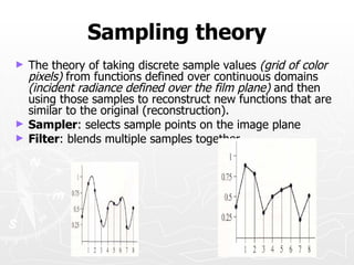
![Unit Step &Unit Impulse
Discrete time Unit impulse is defined as
δ [n]= {0, n≠ 0
{1, n=0
Unit impulse is also known as unit sample.
Discrete time unit step signal is defined by
U[n]={0,n=0
{1,n>= 0
Continuous time unit impulse is defined as
δ (t)={1, t=0
{0, t ≠ 0
Continuous time Unit step signal is defined as
U(t)={0, t<0
{1, t≥0](https://image.slidesharecdn.com/ec2204-nol-120426094244-phpapp02/85/z-transforms-3-320.jpg)
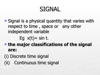
![SIGNAL
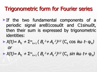
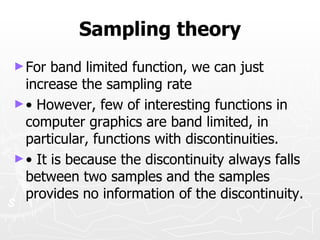
► Periodic Signal & Aperiodic Signal
A signal is said to be periodic ,if it exhibits periodicity.i.e.,
X(t +T)=x(t), for all values of t. Periodic signal has the
property that it is unchanged by a time shift of T. A
signal that does not satisfy the above periodicity property
is called an aperiodic signal
► even and odd signal ?
A discrete time signal is said to be even when, x[-n]=x[n].
The continuous time signal is said to be even when, x(-
t)= x(t) For example,Cosωn is an even signal.](https://image.slidesharecdn.com/ec2204-nol-120426094244-phpapp02/85/z-transforms-4-320.jpg)
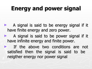

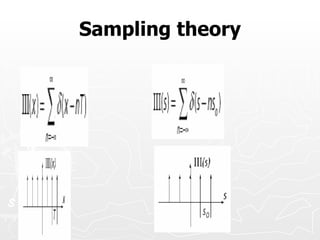
![Convolution
► The input and output signals for LTI
systems have special relationship in terms
of convolution sum and integrals.
► Y(t)=x(t)*h(t) Y[n]=x[n]*h[n]](https://image.slidesharecdn.com/ec2204-nol-120426094244-phpapp02/85/z-transforms-21-320.jpg)

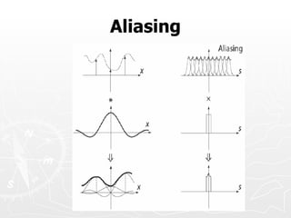
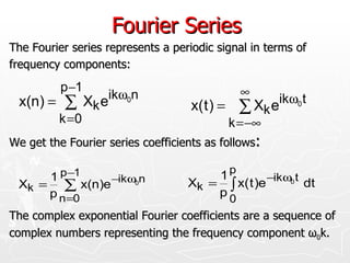
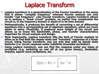
![Z-transforms
► Fordiscrete-time systems, z-transforms play
the same role of Laplace transforms do in
continuous-time systems
Bilateral Forward z-transform Bilateral Inverse z-transform
∞
1
∑ h[ n] z − n
2 π j ∫R
H [ z] = h[n] = H [ z ] z − n +1dz
n = −∞
► Aswith the Laplace transform, we compute
forward and inverse z-transforms by use of
transforms pairs and properties](https://image.slidesharecdn.com/ec2204-nol-120426094244-phpapp02/85/z-transforms-27-320.jpg)

![Z-transform Pairs
► h[n] = δ[n] ► h[n] = an u[n]
∞ 0
∑ δ [ n] z = ∑ δ [ n] z − n = 1
∞
∑ a u[ n] z
−n
H [ z] = H [ z] = n −n
n = −∞ n =0
n = −∞
Region of convergence: ∞
a ∞ n
= ∑ a z = ∑ n −n
entire z-plane n =0 n =0 z
1 a
= if <1
► h[n] ∞= δ[n-1]1 1−
a z
H [ z ] = ∑ δ [ n − 1] z −n = ∑ δ [ n − 1] z −n = z −1 z
n = −∞ n =1
Region of convergence: Region of
entire z-plane convergence: |z|
> |a| which is
h[n-1] ⇔ z-1 H[z]
the complement](https://image.slidesharecdn.com/ec2204-nol-120426094244-phpapp02/85/z-transforms-29-320.jpg)
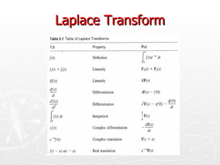
![Stability
► Rule #1: For a causal sequence, poles are
inside the unit circle (applies to z-transform
functions that are ratios of two polynomials)
► Rule #2: More generally, unit circle is
included in region of convergence. (In
continuous-time, the imaginary axis would
be in the region of convergence of the
Z 1
a u[ n] ↔
Laplace transform.)a z for z > a
n
−1
1−
This is stable if |a| < 1 by rule #1.](https://image.slidesharecdn.com/ec2204-nol-120426094244-phpapp02/85/z-transforms-30-320.jpg)
![Inverse z-transform
c + j∞
1
f [ n] = F [ z ] z n −1dz
2πj c∫ j∞
−
► Yuk! Using the definition requires a contour
integration in the complex z-plane.
► Fortunately, we tend to be interested in only
a few basic signals (pulse, step, etc.)
Virtually all of the signals we’ll see can be built
up from these basic signals.
For these common signals, the z-transform pairs
have been tabulated (see Lathi, Table 5.1)](https://image.slidesharecdn.com/ec2204-nol-120426094244-phpapp02/85/z-transforms-31-320.jpg)
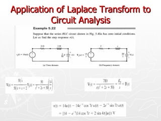
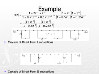
![Example
z 2 + 2z +1 ► Ratio of polynomial z-
X [ z] =
3 1
z2 − z +
2 2
domain functions
1 + 2 z −1 + z −2
► Divide through by the
X [ z] =
3 1
1 − z −1 + z − 2 highest power of z
2 2
► Factor denominator into
1 + 2 z −1 + z −2
X [ z] =
first-order factors
1 − z (1 − z )
1 −1 −1
2 ► Use partial fraction
X [ z ] = B0 +
A1
+
A2 decomposition to get
1 −1 1 − z −1
1− z
2
first-order terms](https://image.slidesharecdn.com/ec2204-nol-120426094244-phpapp02/85/z-transforms-32-320.jpg)
![Example (con’t)
2
1 − 2 3 −1
z − z + 1 z − 2 + 2 z −1 + 1 ► FindB0 by
2 2
z − 2 − 3 z −1 + 2 polynomial division
5 z −1 − 1
− 1 + 5 z −1
X [ z] = 2 +
► Express in terms of
1 −1
1 − z 1 − z
−1
( )
2
B0
1 + 2 z −1 + z −2 1+ 4 + 4
A1 = = = −9
1 − z −1 z −1 = 2
1− 2
1 + 2 z −1 + z − 2 1+ 2 +1
► Solve for A1 and A2
A2 = = =8
1 1
1 − z −1
2 z −1 =1 2](https://image.slidesharecdn.com/ec2204-nol-120426094244-phpapp02/85/z-transforms-33-320.jpg)
![Example (con’t)
► Express X[z] in terms of B0, A1, and A2
9 8
X [ z] = 2 − +
1 −1 1 − z −1
1− z
2
► Use table to obtain inverse z-transform
n
1
x[ n] = 2 δ [ n] − 9 u[ n] + 8 u[ n]
2
► With the unilateral z-transform, or the
bilateral z-transform with region of
convergence, the inverse z-transform is
unique](https://image.slidesharecdn.com/ec2204-nol-120426094244-phpapp02/85/z-transforms-34-320.jpg)
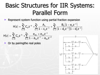
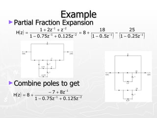
![Z-transform Properties
► Linearity
a1 f1 [ n] + a2 f 2 [ n] ⇔ a1 F1 [ z ] + a2 F2 [ z ]
► Right shift (delay)
f [ n − m] u[ n − m] ⇔ z − m F [ z ]
m
f [ n − m] u[ n] ⇔ z F [ z ] + z ∑ f [ − n] z − n
−m −m
n =1 ](https://image.slidesharecdn.com/ec2204-nol-120426094244-phpapp02/85/z-transforms-35-320.jpg)
![Z-transform Properties
► Convolution definition
∞
f1 [ n] ∗ f 2 [ n] = ∑ f [ m] f [ n − m]
m = −∞
1 2
► Take z-transform
∞
Z { f1 [ n] ∗ f 2 [ n]} = Z ∑ f1 [ m] f 2 [ n − m]
m = −∞
► Z-transform definition
∞
∞
= ∑ ∑ f1 [ m] f 2 [ n − m] z − n ► Interchange summation
n = −∞ m = −∞
∞ ∞
= ∑ f [ m] ∑ f [ n − m] z
1 2
−n ► Substitute r = n - m
m = −∞ n = −∞
∞ ∞
f1 [ m] ∑ f 2 [ r ] z −( r + m )
► Z-transform definition
= ∑
m = −∞ r = −∞
∞
− m
∞
= ∑ f1 [ m]z ∑ f 2 [ r ] z − r
m = −∞ r = −∞
= F1 [ z ] F2 [ z ]](https://image.slidesharecdn.com/ec2204-nol-120426094244-phpapp02/85/z-transforms-36-320.jpg)

![Introduction
► Impulse response h[n] can fully characterize a LTI
system, and we can have the output of LTI system as
y[ n] = x[ n] ∗ h[ n]
► The z-transform of impulse response is called transfer or
Y ( z ) = X ( z ) H ( z ).
system function H(z).
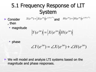
► ( )
Frequency response at H e = H ( z )
jω
z =1
is valid if
z =
ROC includes 1, and
Y ( e jω ) = X ( e jω ) H ( e jω )](https://image.slidesharecdn.com/ec2204-nol-120426094244-phpapp02/85/z-transforms-38-320.jpg)
![System Function
► General formNof LCCDE M
∑ a y [ n − k ] = ∑ b x[ n − k ]
k =0
k
k =0
k
N M
∑ ak z Y ( z ) = ∑ bk z −k X ( z )
−k
k =0 k =0
► Compute the z-transform
M
Y ( z) ∑ bk z −k
H ( z) = = k =0
X ( z) N
∑ ak z − k
k =0](https://image.slidesharecdn.com/ec2204-nol-120426094244-phpapp02/85/z-transforms-40-320.jpg)
![Second-order System
► Suppose the system function of a LTI system is
(1 + z −1 )2
H ( z) = .
1 −1 3 −1
(1 − z )(1 + z )
2 4
► Tofind the difference equation that is satisfied by
the input and out of this system
(1 + z −1 )2 1 + 2 z −1 + z −2 Y ( z)
H ( z) = = =
1 3 1 3
(1 − z −1 )(1 + z −1 ) 1 + z −1 − z −2 X ( z )
2 4 4 8
1 3
y[n ] + y[n − 1] − y[n − 2] = x[n ] + 2 x[n − 1] + 2 x[n − 2]
4 8
► Can we know the impulse response?](https://image.slidesharecdn.com/ec2204-nol-120426094244-phpapp02/85/z-transforms-42-320.jpg)
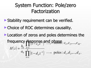
![System Function: Stability
► Stability of LTI system:
∞
∑ h[n] < ∞
n = −∞
► This condition is identical to the condition
∞
that ∑ h[n ]z −n < ∞ when z = 1.
n = −∞
The stability condition is equivalent to the
condition that the ROC of H(z) includes the unit
circle.](https://image.slidesharecdn.com/ec2204-nol-120426094244-phpapp02/85/z-transforms-43-320.jpg)
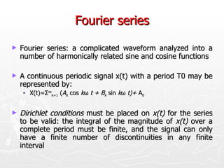
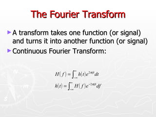
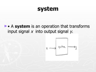
![System Function: Causality
► If the system is causal, it follows that h[n] must be a right-
sided sequence. The ROC of H(z) must be outside the
outermost pole.
► If the system is anti-causal, it follows that h[n] must be a
left-sided sequence. The ROC of H(z) must be inside the
innermost pole.
Im Im Im
a 1 a 1 Re a b
Re Re
Right-sided Left-sided Two-sided
(causal) (anti-causal) (non-causal)](https://image.slidesharecdn.com/ec2204-nol-120426094244-phpapp02/85/z-transforms-44-320.jpg)
![Determining the ROC
► Consider the LTI system
5
y[n ] − y[n − 1] + y[n − 2] = x[n ]
2
► The system1 function is obtained as
H ( z) =
5 −1 −2
1− z +z
2
1
=
1 −1
(1 − z )(1 − 2 z −1 )
2](https://image.slidesharecdn.com/ec2204-nol-120426094244-phpapp02/85/z-transforms-45-320.jpg)
![System Function: Inverse Systems
H i ( z) H ( z)
► is an inverse system for , if
G ( z ) = H ( z ) H i ( z ) = 1 ⇔ g [ n ] = h[ n ] ∗ hi [ n ] = δ [ n ]
1 1
Hi ( z) = jω
⇔ H i (e ) =
H ( z) H ( e jω )
► The ROCs of H ( z ) and H i ( z ) overlap.
must
► Useful for canceling the effects of another system
► See the discussion in Sec.5.2.2 regarding ROC](https://image.slidesharecdn.com/ec2204-nol-120426094244-phpapp02/85/z-transforms-46-320.jpg)


![Example
y[n] = a1y[n − 1] + a2 y[n − 2] + b0x[n]
► Block diagram representation of](https://image.slidesharecdn.com/ec2204-nol-120426094244-phpapp02/85/z-transforms-52-320.jpg)
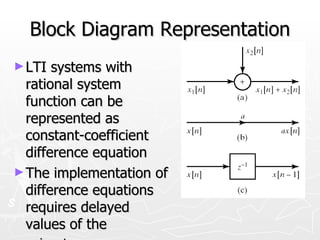
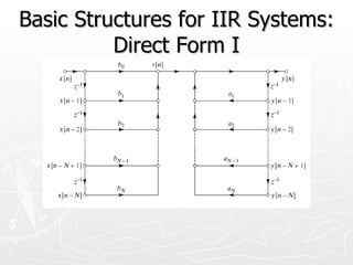
![Direct Form I
N M
∑ ˆ y[n − k ] = ∑ b x[n − k ]
a
k =0
k
ˆ
k =0
k
► General form of difference equation
N M
y[n] − ∑ a y[n − k ] = ∑ b x[n − k ]
k k
k =1 k =0
► Alternative equivalent form](https://image.slidesharecdn.com/ec2204-nol-120426094244-phpapp02/85/z-transforms-54-320.jpg)
![Direct Form I M
∑ bk z −k
H( z ) = k =0
N
1 − ∑ ak z −k
► Transfer function can be written as
k =1
M
H( z ) = H2 ( z )H1 ( z ) = 1 b z −k
∑
N k = 0 k
−k
1 − ∑ ak z
k =1
M −k
V ( z ) = H1 ( z ) X( z ) = ∑ bk z X( z ) M
k =0
v[n] = ∑ b x[n − k ]
k
► Direct Form I Represents
k =0
N
1
y[n] = ∑ a y[n − k ] + v[n]
Y ( z ) = H2 ( z ) V ( z ) = V ( z ) k
k =1
N
1 − ∑ ak z
−k
k =1 ](https://image.slidesharecdn.com/ec2204-nol-120426094244-phpapp02/85/z-transforms-55-320.jpg)
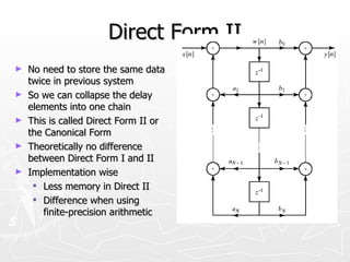
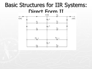
![Alternative Representation
► Replace order of cascade LTI systems
M
1
H( z ) = H ( z )H ( z ) = ∑ b z
−k
1 2
k
1− N
k =0
∑a z
k =1
k
−k
N
w[n] = ∑ a w[n − k ] + x[n]
k
k =1
1
W( z ) = H2 ( z ) X( z ) = X ( z ) M
N y[n] = ∑ b w[n − k ]
k
1 − ∑ ak z
−k
k =0
k =1
M
Y ( z ) = H1 ( z ) W( z ) = ∑ bk z −k W( z )
k =0 ](https://image.slidesharecdn.com/ec2204-nol-120426094244-phpapp02/85/z-transforms-56-320.jpg)
![Alternative Block Diagram
► We can change the order of the cascade
systems
N
w[n] = ∑ a w[n − k ] + x[n]
k
k =1
M
y[n] = ∑ b w[n − k ]
k
k =0](https://image.slidesharecdn.com/ec2204-nol-120426094244-phpapp02/85/z-transforms-57-320.jpg)
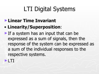
![Example
► Representation of Direct Form II with signal
flow graphs w1 [n] = aw4 [n] + x[n]
w2 [n] = w1 [n]
w3 [n] = b0w2 [n] + b1w4 [n]
w4 [n] = w2 [n − 1]
y[n] = w3 [n]
w1 [n] = aw1 [n − 1] + x[n]
y[n] = b0w1 [n] + b1w1 [n − 1]](https://image.slidesharecdn.com/ec2204-nol-120426094244-phpapp02/85/z-transforms-60-320.jpg)
![Determination of System
Function from Flow Graph
w1 [n] = w4 [n] − x[n]
w2 [n] = αw1 [n]
w3 [n] = w2 [n] + x[n]
w4 [n] = w3 [n − 1]
y[n] = w2 [n] + w4 [n]
W1 ( z ) = W4 ( z ) − X( z ) (
αX( z ) z −1 − 1 )
W2 ( z ) =
W2 ( z ) = αW1 ( z ) 1 − αz −1 Y ( z) z −1 − α
H( z ) = =
W3 ( z ) = W2 ( z ) + X( z ) X( z ) z −1 (1 − α ) X( z ) 1 − αz −1
W4 ( z ) =
W4 ( z ) = W3 ( z ) z −1 1 − αz −1 h[n] = αn −1u[n − 1] − αn +1u[n]
Y ( z ) = W2 ( z ) + W4 ( z ) Y ( z ) = W2 ( z ) + W4 ( z )](https://image.slidesharecdn.com/ec2204-nol-120426094244-phpapp02/85/z-transforms-61-320.jpg)
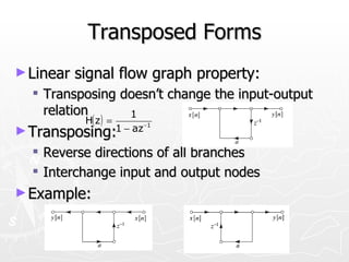
![Example
Transpose
y[n] = a1y[n − 1] + a2y[n − 2] + b0x[n] + b1x[n − 1] + b2x[n − 2]
► Both have the same system function or
difference equation](https://image.slidesharecdn.com/ec2204-nol-120426094244-phpapp02/85/z-transforms-69-320.jpg)
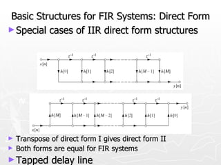
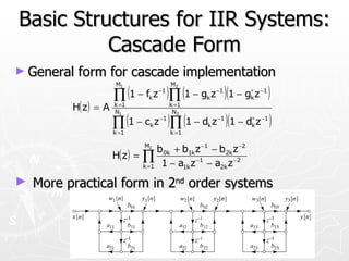
![Basic Structures for FIR Systems:
Cascade Form
► Obtainedby factoring the polynomial
system function
MS
∏ (b )
M
H( z ) = ∑ h[n]z
n=0
−n
=
k =1
0k + b1k z −1 + b2k z −2](https://image.slidesharecdn.com/ec2204-nol-120426094244-phpapp02/85/z-transforms-71-320.jpg)
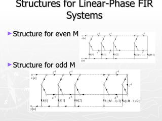
![Structures for Linear-Phase FIR
Systems
► Causal FIR system with generalized linear phase are
symmetric:
h[M − n] = h[n] n = 0,1,..., M (type I or III)
h[M − n] = −h[n] n = 0,1,..., M (type II or IV)
► Symmetry means we can half the number of
multiplications
► Example: For even M and type I or type III systems:
M M / 2 −1 M
y[n] = ∑ h[k ]x[n − k ] = ∑ h[k ]x[n − k ] + h[M / 2]x[n − M / 2] + ∑ h[k ]x[n − k ]
k =0 k =0 k = M / 2 +1
M / 2 −1 M / 2 −1
= ∑ h[k ]x[n − k ] + h[M / 2]x[n − M / 2] + ∑ h[M − k ]x[n − M + k ]
k =0 k =0
M / 2 −1
= ∑ h[k ]( x[n − k ] + x[n − M + k ] ) + h[M / 2]x[n − M / 2]
k =0](https://image.slidesharecdn.com/ec2204-nol-120426094244-phpapp02/85/z-transforms-72-320.jpg)

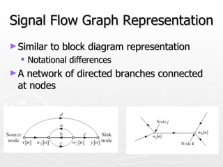
This document discusses signals and systems. It defines signals as physical quantities that vary with respect to time, space, or another independent variable. Signals can be classified as discrete time or continuous time. It also defines unit impulse and unit step functions for discrete and continuous time. Periodic and aperiodic signals are discussed. The Fourier series and Fourier transform are introduced as ways to represent signals in the frequency domain. The Laplace transform, which generalizes the Fourier transform, is also mentioned. Key properties of linear time-invariant systems like superposition, time-invariance, and convolution are covered. Finally, sampling theory and the z-transform, which is analogous to the Laplace transform for discrete-time systems, are summarized at a high level


![Digital Signal Processing[ECEG-3171]-Ch1_L03](https://cdn.slidesharecdn.com/ss_thumbnails/dspl3-180427094423-thumbnail.jpg?width=640&height=640&fit=bounds)