We present an ab-initio real-time based computational approach to nonlinear optical properties in Condensed Matter systems. The equation of mot ions, and in particular the coupling of the electrons with the external electric field, are derived from the Berry phase formulation of the dynamical polarization. The zero-field Hamiltonian includes crystal local field effects, the renormalization of the independent particle energy levels by correlation and excitonic effects within the screened Hartree- Fock self-energy operator. The approach is validated by calculating the second-harmonic generation of SiC and AlAs bulk semiconductors : an excellent agreement is obtained with existing ab-initio calculations from response theory in frequency domain . We finally show applications to the second-harmonic generation of CdTe the third-harmonic generation of Si.
Reference :
Real-time approach to the optical properties of solids and nanostructures : Time-dependent Bethe-alpeter equation Phys. Rev. B 84, 245110 (2011)
Nonlinear optics from ab-initio by means of the dynamical Berry-phase
C. Attaccalite and M. Gruning Phys. Rev. B 88 (23), 235113 (2013)
NANO106 is UCSD Department of NanoEngineering's core course on crystallography of materials taught by Prof Shyue Ping Ong. For more information, visit the course wiki at http://nano106.wikispaces.com.
II. Charge transport and nanoelectronics.
Quantum Hall Effect: 2D electron gas (2DEG) in magnetic field, Landau levels, de Haas-van Alphen and Shubnikov-de Haas Effects, integer and fractional quantum Hall effects, Spin Hall Effect.
Quantum transport: Transport regimes and mesoscopic quantum transport, Scattering theory of conductance and Landauer-Buttiker formalism, Quantum point contacts, Quantum electronics and selected examples of mesoscopic devices (quantum interference devices).
Tunneling: Scanning tunneling microscopy and spectroscopy (and wavefunction mapping in nanostructures and molecules), Nanoelectronic devices based on tunneling, Coulomb blockade, Single electron transistors, Kondo effect.
Molecular electronics: Donor-Acceptor systems, Nanoscale charge transfer, Electronic properties and transport in molecules and biomolecules; single molecule transistors.
The resistivity of a host metal, such as Cu with trace amounts of magnetic impurities, typically Fe, reaches a minimum and then increases as -ln T as the temperature subsequently decreases. A resistivity minimum and subsequent logarithmic-temperature dependence are in stark contrast to the resistivity of the pure metal that tends to zero monotonically as the temperature decreases. An additional surprise is that the -ln T dependence of the resistivity does not continue indefinitely to low temperature, but rather, below a characteristic temperature, the Kondo temperature, it phases out. At this temperature the impurity and conduction electron spins begin to condense into singlet states and this condensation is complete at T=0 K. Perturbation theory breaks down at this temperature and then the magnetic properties of the system change. Here we have explained how resistivity minimum and logarithmic-temperature dependence arises if we take the interaction between the spin of conduction electrons of host metal and the spin of impurity as a perturbation.
The integral & fractional quantum hall effectSUDIPTO DAS
Introductory idea of integral & fractional quantum hall effect and by imposing the idea of composite fermions showing the existence of fractional charge.
Microscopic Mechanisms of Superconducting Flux Quantum and Superconducting an...Qiang LI
We have provided microscopic explanations to superconducting flux quantum and (superconducting and normal) persistent current. Flux quantum is generated by current carried by "deep electrons" at surface states. And values of the flux quantum differs according to the electronic states and coupling of the carrier electrons. Generation of persistent carrier electrons does not dissipate energy; instead there would be emission of real phonons and release of corresponding energy into the environment; but the normal carrier electrons involved still dissipate energy. Even for or persistent carriers,there should be a build-up of energy of the middle state and a build-up of the probability of virtual transition of electrons to the middle state, and the corresponding relaxation should exist accordingly.
UCSD NANO 266 Quantum Mechanical Modelling of Materials and Nanostructures is a graduate class that provides students with a highly practical introduction to the application of first principles quantum mechanical simulations to model, understand and predict the properties of materials and nano-structures. The syllabus includes: a brief introduction to quantum mechanics and the Hartree-Fock and density functional theory (DFT) formulations; practical simulation considerations such as convergence, selection of the appropriate functional and parameters; interpretation of the results from simulations, including the limits of accuracy of each method. Several lab sessions provide students with hands-on experience in the conduct of simulations. A key aspect of the course is in the use of programming to facilitate calculations and analysis.
Is ellipse really a section of cone. The question intrigued me for 20 odd years after leaving high school. Finally got the proof on a cremation ground. Only thereafter I came to know of Dandelin spheres. But this proof uses only bare basics within the scope of high school course of Analytical geometry.
Bound State Solution of the Klein–Gordon Equation for the Modified Screened C...BRNSS Publication Hub
We present solution of the Klein–Gordon equation for the modified screened Coulomb potential (Yukawa) plus inversely quadratic Yukawa potential through formula method. The conventional formula method which constitutes a simple formula for finding bound state solution of any quantum mechanical wave equation, which is simplified to the form; 2122233()()''()'()()0(1)(1)kksAsBscsssskssks−++ψ+ψ+ψ=−−. The bound state energy eigenvalues and its corresponding wave function obtained with its efficiency in spectroscopy.
Key words: Bound state, inversely quadratic Yukawa, Klein–Gordon, modified screened coulomb (Yukawa), quantum wave equation
I am Geoffrey J. I am a Stochastic Processes Homework Expert at excelhomeworkhelp.com. I hold a Ph.D. in Statistics, from Edinburgh, UK. I have been helping students with their homework for the past 6 years. I solve homework related to Stochastic Processes. Visit excelhomeworkhelp.com or email info@excelhomeworkhelp.com. You can also call on +1 678 648 4277 for any assistance with Stochastic Processes Homework.
Question answers Optical Fiber Communications 4th Edition by Keiserblackdance1
Scribd download slideshare Solution manual Optical Fiber Communications 4th Edition by Keiser Full Download link at https://findtestbanks.com/download/solution-manual-optical-fiber-communications-4th-edition-by-keiser/ instant download communication systems,fiber communications 4th,Gerd Keiser,optical fiber
This is downloadable version of Solution manual Optical Fiber Communications 4th Edition by Gerd Keiser
Instant download Optical Fiber Communications 4th Edition solutions after payment item
Solution manual Optical Fiber Communications 4th Edition by Gerd Keiser
Click link bellow to view sample chapter of Optical Fiber Communications 4th solutions
http://findtestbanks.com/wp-content/uploads/2017/06/Link-download-Solution-manual-Optical-Fiber-Communications-4th-Edition-by-Gerd-Keiser.pdf
The fou free solution and test banks list
Similar to Kittel c. introduction to solid state physics 8 th edition - solution manual (20)
Slide 1: Title Slide
Extrachromosomal Inheritance
Slide 2: Introduction to Extrachromosomal Inheritance
Definition: Extrachromosomal inheritance refers to the transmission of genetic material that is not found within the nucleus.
Key Components: Involves genes located in mitochondria, chloroplasts, and plasmids.
Slide 3: Mitochondrial Inheritance
Mitochondria: Organelles responsible for energy production.
Mitochondrial DNA (mtDNA): Circular DNA molecule found in mitochondria.
Inheritance Pattern: Maternally inherited, meaning it is passed from mothers to all their offspring.
Diseases: Examples include Leber’s hereditary optic neuropathy (LHON) and mitochondrial myopathy.
Slide 4: Chloroplast Inheritance
Chloroplasts: Organelles responsible for photosynthesis in plants.
Chloroplast DNA (cpDNA): Circular DNA molecule found in chloroplasts.
Inheritance Pattern: Often maternally inherited in most plants, but can vary in some species.
Examples: Variegation in plants, where leaf color patterns are determined by chloroplast DNA.
Slide 5: Plasmid Inheritance
Plasmids: Small, circular DNA molecules found in bacteria and some eukaryotes.
Features: Can carry antibiotic resistance genes and can be transferred between cells through processes like conjugation.
Significance: Important in biotechnology for gene cloning and genetic engineering.
Slide 6: Mechanisms of Extrachromosomal Inheritance
Non-Mendelian Patterns: Do not follow Mendel’s laws of inheritance.
Cytoplasmic Segregation: During cell division, organelles like mitochondria and chloroplasts are randomly distributed to daughter cells.
Heteroplasmy: Presence of more than one type of organellar genome within a cell, leading to variation in expression.
Slide 7: Examples of Extrachromosomal Inheritance
Four O’clock Plant (Mirabilis jalapa): Shows variegated leaves due to different cpDNA in leaf cells.
Petite Mutants in Yeast: Result from mutations in mitochondrial DNA affecting respiration.
Slide 8: Importance of Extrachromosomal Inheritance
Evolution: Provides insight into the evolution of eukaryotic cells.
Medicine: Understanding mitochondrial inheritance helps in diagnosing and treating mitochondrial diseases.
Agriculture: Chloroplast inheritance can be used in plant breeding and genetic modification.
Slide 9: Recent Research and Advances
Gene Editing: Techniques like CRISPR-Cas9 are being used to edit mitochondrial and chloroplast DNA.
Therapies: Development of mitochondrial replacement therapy (MRT) for preventing mitochondrial diseases.
Slide 10: Conclusion
Summary: Extrachromosomal inheritance involves the transmission of genetic material outside the nucleus and plays a crucial role in genetics, medicine, and biotechnology.
Future Directions: Continued research and technological advancements hold promise for new treatments and applications.
Slide 11: Questions and Discussion
Invite Audience: Open the floor for any questions or further discussion on the topic.
THE IMPORTANCE OF MARTIAN ATMOSPHERE SAMPLE RETURN.Sérgio Sacani
The return of a sample of near-surface atmosphere from Mars would facilitate answers to several first-order science questions surrounding the formation and evolution of the planet. One of the important aspects of terrestrial planet formation in general is the role that primary atmospheres played in influencing the chemistry and structure of the planets and their antecedents. Studies of the martian atmosphere can be used to investigate the role of a primary atmosphere in its history. Atmosphere samples would also inform our understanding of the near-surface chemistry of the planet, and ultimately the prospects for life. High-precision isotopic analyses of constituent gases are needed to address these questions, requiring that the analyses are made on returned samples rather than in situ.
The increased availability of biomedical data, particularly in the public domain, offers the opportunity to better understand human health and to develop effective therapeutics for a wide range of unmet medical needs. However, data scientists remain stymied by the fact that data remain hard to find and to productively reuse because data and their metadata i) are wholly inaccessible, ii) are in non-standard or incompatible representations, iii) do not conform to community standards, and iv) have unclear or highly restricted terms and conditions that preclude legitimate reuse. These limitations require a rethink on data can be made machine and AI-ready - the key motivation behind the FAIR Guiding Principles. Concurrently, while recent efforts have explored the use of deep learning to fuse disparate data into predictive models for a wide range of biomedical applications, these models often fail even when the correct answer is already known, and fail to explain individual predictions in terms that data scientists can appreciate. These limitations suggest that new methods to produce practical artificial intelligence are still needed.
In this talk, I will discuss our work in (1) building an integrative knowledge infrastructure to prepare FAIR and "AI-ready" data and services along with (2) neurosymbolic AI methods to improve the quality of predictions and to generate plausible explanations. Attention is given to standards, platforms, and methods to wrangle knowledge into simple, but effective semantic and latent representations, and to make these available into standards-compliant and discoverable interfaces that can be used in model building, validation, and explanation. Our work, and those of others in the field, creates a baseline for building trustworthy and easy to deploy AI models in biomedicine.
Bio
Dr. Michel Dumontier is the Distinguished Professor of Data Science at Maastricht University, founder and executive director of the Institute of Data Science, and co-founder of the FAIR (Findable, Accessible, Interoperable and Reusable) data principles. His research explores socio-technological approaches for responsible discovery science, which includes collaborative multi-modal knowledge graphs, privacy-preserving distributed data mining, and AI methods for drug discovery and personalized medicine. His work is supported through the Dutch National Research Agenda, the Netherlands Organisation for Scientific Research, Horizon Europe, the European Open Science Cloud, the US National Institutes of Health, and a Marie-Curie Innovative Training Network. He is the editor-in-chief for the journal Data Science and is internationally recognized for his contributions in bioinformatics, biomedical informatics, and semantic technologies including ontologies and linked data.
Nutraceutical market, scope and growth: Herbal drug technologyLokesh Patil
As consumer awareness of health and wellness rises, the nutraceutical market—which includes goods like functional meals, drinks, and dietary supplements that provide health advantages beyond basic nutrition—is growing significantly. As healthcare expenses rise, the population ages, and people want natural and preventative health solutions more and more, this industry is increasing quickly. Further driving market expansion are product formulation innovations and the use of cutting-edge technology for customized nutrition. With its worldwide reach, the nutraceutical industry is expected to keep growing and provide significant chances for research and investment in a number of categories, including vitamins, minerals, probiotics, and herbal supplements.
Earliest Galaxies in the JADES Origins Field: Luminosity Function and Cosmic ...Sérgio Sacani
We characterize the earliest galaxy population in the JADES Origins Field (JOF), the deepest
imaging field observed with JWST. We make use of the ancillary Hubble optical images (5 filters
spanning 0.4−0.9µm) and novel JWST images with 14 filters spanning 0.8−5µm, including 7 mediumband filters, and reaching total exposure times of up to 46 hours per filter. We combine all our data
at > 2.3µm to construct an ultradeep image, reaching as deep as ≈ 31.4 AB mag in the stack and
30.3-31.0 AB mag (5σ, r = 0.1” circular aperture) in individual filters. We measure photometric
redshifts and use robust selection criteria to identify a sample of eight galaxy candidates at redshifts
z = 11.5 − 15. These objects show compact half-light radii of R1/2 ∼ 50 − 200pc, stellar masses of
M⋆ ∼ 107−108M⊙, and star-formation rates of SFR ∼ 0.1−1 M⊙ yr−1
. Our search finds no candidates
at 15 < z < 20, placing upper limits at these redshifts. We develop a forward modeling approach to
infer the properties of the evolving luminosity function without binning in redshift or luminosity that
marginalizes over the photometric redshift uncertainty of our candidate galaxies and incorporates the
impact of non-detections. We find a z = 12 luminosity function in good agreement with prior results,
and that the luminosity function normalization and UV luminosity density decline by a factor of ∼ 2.5
from z = 12 to z = 14. We discuss the possible implications of our results in the context of theoretical
models for evolution of the dark matter halo mass function.
Cancer cell metabolism: special Reference to Lactate PathwayAADYARAJPANDEY1
Normal Cell Metabolism:
Cellular respiration describes the series of steps that cells use to break down sugar and other chemicals to get the energy we need to function.
Energy is stored in the bonds of glucose and when glucose is broken down, much of that energy is released.
Cell utilize energy in the form of ATP.
The first step of respiration is called glycolysis. In a series of steps, glycolysis breaks glucose into two smaller molecules - a chemical called pyruvate. A small amount of ATP is formed during this process.
Most healthy cells continue the breakdown in a second process, called the Kreb's cycle. The Kreb's cycle allows cells to “burn” the pyruvates made in glycolysis to get more ATP.
The last step in the breakdown of glucose is called oxidative phosphorylation (Ox-Phos).
It takes place in specialized cell structures called mitochondria. This process produces a large amount of ATP. Importantly, cells need oxygen to complete oxidative phosphorylation.
If a cell completes only glycolysis, only 2 molecules of ATP are made per glucose. However, if the cell completes the entire respiration process (glycolysis - Kreb's - oxidative phosphorylation), about 36 molecules of ATP are created, giving it much more energy to use.
IN CANCER CELL:
Unlike healthy cells that "burn" the entire molecule of sugar to capture a large amount of energy as ATP, cancer cells are wasteful.
Cancer cells only partially break down sugar molecules. They overuse the first step of respiration, glycolysis. They frequently do not complete the second step, oxidative phosphorylation.
This results in only 2 molecules of ATP per each glucose molecule instead of the 36 or so ATPs healthy cells gain. As a result, cancer cells need to use a lot more sugar molecules to get enough energy to survive.
introduction to WARBERG PHENOMENA:
WARBURG EFFECT Usually, cancer cells are highly glycolytic (glucose addiction) and take up more glucose than do normal cells from outside.
Otto Heinrich Warburg (; 8 October 1883 – 1 August 1970) In 1931 was awarded the Nobel Prize in Physiology for his "discovery of the nature and mode of action of the respiratory enzyme.
WARNBURG EFFECT : cancer cells under aerobic (well-oxygenated) conditions to metabolize glucose to lactate (aerobic glycolysis) is known as the Warburg effect. Warburg made the observation that tumor slices consume glucose and secrete lactate at a higher rate than normal tissues.
Comparative structure of adrenal gland in vertebrates
Kittel c. introduction to solid state physics 8 th edition - solution manual
1. CHAPTER 1
1. The vectors ˆ ˆ ˆ+ +x y z and ˆ ˆ ˆ− − +x y z are in the directions of two body diagonals of a
cube. If θ is the angle between them, their scalar product gives cos θ = –1/3, whence
.1
cos 1/3 90 19 28' 109 28'−
θ = = °+ ° = °
2. The plane (100) is normal to the x axis. It intercepts the a' axis at and the c' axis
at ; therefore the indices referred to the primitive axes are (101). Similarly, the plane
(001) will have indices (011) when referred to primitive axes.
2a'
2c'
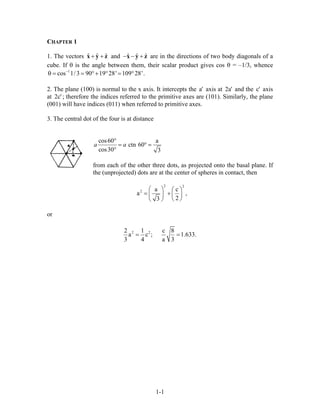
3. The central dot of the four is at distance
cos60 a
ctn 60
cos30 3
a a
°
= ° =
°
from each of the other three dots, as projected onto the basal plane. If
the (unprojected) dots are at the center of spheres in contact, then
2 2
2 a c
a ,
23
⎛ ⎞ ⎛ ⎞
= + ⎜ ⎟⎜ ⎟
⎝ ⎠⎝ ⎠
or
2 22 1 c 8
a c ; 1.633.
3 4 a 3
= =
1-1
2. CHAPTER 2
1. The crystal plane with Miller indices hk is a plane defined by the points a1/h, a2/k, and . (a)
Two vectors that lie in the plane may be taken as a
3 /a
1/h – a2/k and 1 3/ h /−a a . But each of these vectors
gives zero as its scalar product with 1 2h k 3= + +G a a a , so that G must be perpendicular to the plane
. (b) If is the unit normal to the plane, the interplanar spacing ishk ˆn 1
ˆ /h⋅n a . But ,
whence . (c) For a simple cubic lattice
ˆ / | |=n G G
1d(hk ) G / h| | 2 / | G|= ⋅ = πa G ˆ ˆ ˆ(2 / a)(h k )= π + +G x y z ,
whence
2 2 2 2
2 2 2
1 G h k
.
d 4 a
+ +
= =
π
1 2 3
1 1
3a a 0
2 2
1 1
2. (a) Cell volume 3a a 0
2 2
0 0
⋅ × = −a a a
c
21
3 a c.
2
=
2 3
1 2
1 2 3
2 3
ˆ ˆ
4 1 1
(b) 2 3a a 0
| | 2 23a c
0 0
2 1
ˆ ˆ( ), and similarly for , .
a 3
× π
= π = −
⋅ ×
π
= +
x ˆ
c
y z
a a
b
a a a
x y b b
(c) Six vectors in the reciprocal lattice are shown as solid lines. The broken
lines are the perpendicular bisectors at the midpoints. The inscribed hexagon
forms the first Brillouin Zone.
3. By definition of the primitive reciprocal lattice vectors
3 32 3 3 1 1 2
1 2 33
1 2 3
3
C
(a a ) (a a ) (a a )
) (2 ) / | (a a a ) |
| (a a a ) |
/ V .
BZV (2
(2 )
× ⋅ × × ×
= π ⋅ ×
⋅ ×
= π
= π
For the vector identity, see G. A. Korn and T. M. Korn, Mathematical handbook for scientists and
engineers, McGraw-Hill, 1961, p. 147.
4. (a) This follows by forming
2-1
3. 2
2 1
2
2 1
2
1 exp[ iM(a k)] 1 exp[iM(a k)]
|F|
1 exp[ i(a k)] 1 exp[i(a k)]
sin M(a k)1 cosM(a k)
.
1 cos(a k) sin (a k)
− − ⋅ ∆ − ⋅ ∆
= ⋅
− − ⋅ ∆ − ⋅ ∆
⋅ ∆− ⋅ ∆
= =
− ⋅ ∆ ⋅ ∆
(b) The first zero in
1
sin M
2
ε occurs for ε = 2π/M. That this is the correct consideration follows from
1zero,
as Mh is
an integer
1 1
sin M( h ) sin Mh cos M cos Mh sin M .
2 2 ±
π + ε = π ε + π ε
1
2
5. j 1 j 2 j 32 i(x v +y v +z v )
1 2 3S (v v v ) f e
j
− π
= Σ
Referred to an fcc lattice, the basis of diamond is
1 1 1
000; .
4 4 4
Thus in the product
1 2 3S(v v v ) S(fcc lattice) S (basis)= × ,
we take the lattice structure factor from (48), and for the basis
1 2 3
1
i (v v v ).
2
S (basis) 1 e
− π + +
= +
Now S(fcc) = 0 only if all indices are even or all indices are odd. If all indices are even the structure factor
of the basis vanishes unless v1 + v2 + v3 = 4n, where n is an integer. For example, for the reflection (222)
we have S(basis) = 1 + e–i3π
= 0, and this reflection is forbidden.
32 1
G 0
0
33
0 0
3 23 2 2
0 0 0
22 2
0
6. f 4 r ( a Gr) sin Gr exp ( 2r a ) dr
(4 G a ) dx x sin x exp ( 2x Ga )
(4 G a ) (4 Ga ) (1 r G a )
16 (4 G a ) .
∞
−
= π π −
= −
= +
+
∫
∫
0
The integral is not difficult; it is given as Dwight 860.81. Observe that f = 1 for G = 0 and f ∝ 1/G4
for
0Ga 1.>>
7. (a) The basis has one atom A at the origin and one atom
1
B at a.
2
The single Laue equation
defines a set of parallel planes in Fourier space. Intersections with a sphere are
a set of circles, so that the diffracted beams lie on a set of cones. (b) S(n) = f
2 (integer)⋅∆ π×a k =
A + fB e–iπn
. For n odd, S = fA –
2-2
4. fB; for n even, S = fA + fB. (c) If fA = fB the atoms diffract identically, as if the primitive translation vector
were
1
a
2
and the diffraction condition
1
( ) 2 (integer).
2
⋅∆ = π ×a k
2-3
5. CHAPTER 3
1.
2 2 2 2
E (h 2M) (2 ) (h 2M) ( L) , with 2L/ /= π λ = π λ .=
2. bcc:
12 6
U(R) 2N [9.114( R ) 12.253( R) ].= ε σ − σ At equilibrium and
6 6
0R 1.488= σ ,
0U(R ) 2N ( 2.816).= ε −
fcc:
12 6
U(R) 2N [12.132( R ) 14.454( R) ].= ε σ − σ At equilibrium and
Thus the cohesive energy ratio bcc/fcc = 0.956, so that the fcc structure is
more stable than the bcc.
6 6
0R 1.679= σ ,
0U(R ) 2N ( 4.305).= ε −
23 16 9
3. | U | 8.60 N
(8.60)(6.02 10 ) (50 10 ) 25.9 10 erg mol
2.59 kJ mol.
−
= ε
= × × = ×
=
This will be decreased significantly by quantum corrections, so that it is quite reasonable to find the same
melting points for H2 and Ne.
4. We have Na → Na+
+ e – 5.14 eV; Na + e → Na–
+ 0.78 eV. The Madelung energy in the NaCl
structure, with Na+
at the Na+
sites and Na–
at the Cl–
sites, is
2 10 2
12
8
e (1.75) (4.80 10 )
11.0 10 erg,
R 3.66 10
−
−
−
α ×
= = ×
×
or 6.89 eV. Here R is taken as the value for metallic Na. The total cohesive energy of a Na+
Na–
pair in the
hypothetical crystal is 2.52 eV referred to two separated Na atoms, or 1.26 eV per atom. This is larger than
the observed cohesive energy 1.13 eV of the metal. We have neglected the repulsive energy of the Na+
Na–
structure, and this must be significant in reducing the cohesion of the hypothetical crystal.
5a.
2
n
A q
U(R) N ; 2 log 2 Madelung const.
R R
⎛ ⎞α
= − α = =⎜ ⎟
⎝ ⎠
In equilibrium
2
n
02n 1 2
0 0
U nA q n
N 0 ; R
R R R
+
⎛ ⎞∂ α
= − + = =⎜ ⎟
∂ α⎝ ⎠
A
,
q
and
2
0
0
N q 1
U(R ) (1 ).
R n
α
= − −
3-1
6. b. ( ) ( )
2
2
0 0 0 0 02
1 U
U(R -R ) U R R R ...,
2 R
∂
δ = + δ +
∂
bearing in mind that in equilibrium R
0
( U R) 0.∂ ∂ =
2 2
n 2 3 3 32
0 0 0
0
U n(n 1)A 2 q (n 1) q 2
N N
R R R R RR
2
+
⎛ ⎞ ⎛⎛ ⎞∂ + α + α
= − = −⎜ ⎟ ⎜⎜ ⎟
∂⎝ ⎠ ⎝ ⎠ ⎝
2
0
q ⎞α
⎟
⎠
For a unit length 2NR0 = 1, whence
0
2 2 2 2
2
04 22 2
0 0R
0
R
U q U (n 1)q log 2
(n 1) ; C R
R R2R R
⎛ ⎞∂ α ∂ −
= − = =⎜ ⎟
∂ ∂⎝ ⎠
.
6. For KCl, λ = 0.34 × 10⁻⁸
ergs and ρ = 0.326 × 10⁻⁸
Å. For the imagined modification of KCl with the
ZnS structure, z = 4 and α = 1.638. Then from Eq. (23) with x ≡ R0/ρ we have
2 x 3
x e 8.53 10 .− −
= ×
By trial and error we find or Rx 9.2, 0 = 3.00 Å. The actual KCl structure has R0 (exp) = 3.15 Å . For
the imagined structure the cohesive energy is
2
2
0 0
-αq p U
U= 1- , or =-0.489
R R q
⎛ ⎞
⎜ ⎟
⎝ ⎠
in units with R0 in Å. For the actual KCl structure, using the data of Table 7, we calculate 2
U
0.495,
q
= −
units as above. This is about 0.1% lower than calculated for the cubic ZnS structure. It is noteworthy that
the difference is so slight.
7. The Madelung energy of Ba+
O–
is –αe2
/R0 per ion pair, or –14.61 × 10⁻¹²
erg = –9.12 eV, as compared
with –4(9.12) = –36.48 eV for Ba++
O--
. To form Ba+
and O–
from Ba and O requires 5.19 – 1.5 = 3.7 eV;
to form Ba++
and O--
requires 5.19 + 9.96 – 1.5 + 9.0 = 22.65 eV. Thus at the specified value of R0 the
binding of Ba+
O–
is 5.42 eV and the binding of Ba++
O--
is 13.83 eV; the latter is indeed the stable form.
8. From (37) we have eXX = S11XX, because all other stress components are zero. By (51),
11 11 12 11 123S 2 (C C ) 1 (C C ).= − + +
Thus
2 2
11 12 11 12 11 12Y (C C C 2C ) (C C );= + − +
further, also from (37), eyy = S21Xx,
whence yy 21 11 12 11 12xx
e e S S C (C C )σ = = = − + .
9. For a longitudinal phonon with K || [111], u = v = w.
3-2
7. 2 2
11 44 12 44
1 2
11 12 44
[C 2C 2(C C )]K 3,
or v K [(C 2C 4C 3 )]ρ
ω ρ = + + +
= ω = + +
This dispersion relation follows from (57a).
10. We take u = – w; v = 0. This displacement is ⊥ to the [111] direction. Shear waves are degenerate in
this direction. Use (57a).
11. Let 1
2xx yye e= − = e in (43). Then
2 21 1 1 1
2 4 4 411 12
21 1
2 2 11 12
U C ( e e ) C e
[ (C C )]e
= + −
= −
2
so that
2 2
n 2 3 3 32
0 0 0
0
U n(n 1)A 2 q (n 1) q 2
N N
R R R R RR
2
+
⎛ ⎞ ⎛⎛ ⎞∂ + α + α
= − = −⎜ ⎟ ⎜⎜ ⎟
∂⎝ ⎠ ⎝ ⎠ ⎝
2
0
q ⎞α
⎟
⎠
is the effective shear
constant.
12a. We rewrite the element aij = p – δ
ij(λ + p – q) as aij = p – λ′ δ
ij, where λ′ = λ + p – q, and δ
ij is the
Kronecker delta function. With λ′ the matrix is in the “standard” form. The root λ′ = Rp gives λ = (R – 1)p
+ q, and the R – 1 roots λ′ = 0 give λ = q – p.
b. Set
i[(K 3) (x y z) t]
0
i[. . . . .]
0
i[. . . . .]
0
u (r, t) u e ;
v(r,t) v e ;
w(r,t) w e ,
+ + −ω
=
=
=
as the displacements for waves in the [111] direction. On substitution in (57) we obtain the desired
equation. Then, by (a), one root is
2 2
11 12 442p q K (C 2C 4C )/3,ω ρ = + = + +
and the other two roots (shear waves) are
2 2
11 12 44K (C C C )/3.ω ρ = − +
13. Set u(r,t) = u0ei(K
·r – t)
and similarly for v and w. Then (57a) becomes
2 2 22
0 11 y 44 y z
12 44 x y 0 x z 0
u [C K C (K K )]u
(C C ) (K K v K K w )
ω ρ = + +
+ + +
0
and similarly for (57b), (57c). The elements of the determinantal equation are
3-3
8. 2 2 2 2
11 11 x 44 y z
12 12 44 x y
13 12 44 x z
M C K C (K K )
M (C C )K K ;
M (C C )K K .
ω ρ;= + + −
= +
= +
and so on with appropriate permutations of the axes. The sum of the three roots of
2
ω ρ is equal to the
sum of the diagonal elements of the matrix, which is
(C11 + 2C44)K2
, where
2 2 22
x y z
2 2 2
1 2 3 11 44
K K K K , whence
v v v (C 2C ) ,ρ
= + +
+ + = +
for the sum of the (velocities)2
of the 3 elastic modes in any direction of K.
14. The criterion for stability of a cubic crystal is that all the principal minors of the quadratic form be
positive. The matrix is:
C11 C12 C12
C12 C11 C12
C12 C12 C11
C44
C44
C44
The principal minors are the minors along the diagonal. The first three minors from the bottom are C44,
C44
2
, C44
3
; thus one criterion of stability is C44 > 0. The next minor is
C11 C44
3
, or C11 > 0. Next: C44
3
(C11
2
– C12
2
), whence |C12| < C11. Finally, (C11 + 2C12) (C11 – C12)2
> 0, so
that C11 + 2C12 > 0 for stability.
3-4
9. CHAPTER 4
1a. The kinetic energy is the sum of the individual kinetic energies each of the form
2
S
1
Mu .
2
The force
between atoms s and s+1 is –C(us – us+1); the potential energy associated with the stretching of this bond is
2
s 1
1
C(u u )
2
s+− , and we sum over all bonds to obtain the total potential energy.
b. The time average of
2 2 2
S
1 1
Mu is M u .
2 4
ω In the potential energy we have
s 1u u cos[ t (s 1)Ka] u{cos( t sKa) cos Ka
sin ( t sKa) sin Ka}.
+ = ω − + = ω − ⋅
+ ω − ⋅
s s 1Then u u u {cos( t sKa) (1 cos Ka)
sin ( t sKa) sin Ka}.
+− = ω − ⋅ −
− ω − ⋅
We square and use the mean values over time:
2 2 1
cos sin ; cos sin 0.
2
< > = < > = < > =
Thus the square of u{} above is
2 2 2 21
u [1 2cos Ka cos Ka sin Ka] u (1 cos Ka).
2
− + + = −
The potential energy per bond is
21
Cu (1 cos Ka),
2
− and by the dispersion relation ω2
= (2C/M) (1 –
cos Ka)
2 21
this is equal to M u .
4
ω Just as for a simple harmonic oscillator, the time average potential
energy is equal to the time-average kinetic energy.
2. We expand in a Taylor series
2
2 2
2
s s
u 1 u
u(s p) u(s) pa p a ;
x 2 x
⎛ ⎞∂ ∂⎛ ⎞
+ = + + +⎜ ⎟⎜ ⎟
∂ ∂⎝ ⎠ ⎝ ⎠
On substitution in the equation of motion (16a) we have
2 2
2 2
p2 2
p 0
u u
M ( p a C )
t x>
∂ ∂
= Σ
∂ ∂
,
which is of the form of the continuum elastic wave equation with
4-1
10. 2 1 2 2
p
p 0
v M p a C−
>
= Σ .
3. From Eq. (20) evaluated at K = π/a, the zone boundary, we have
2
1
2
2
M u 2Cu ;
M v 2Cv .
−ω = −
−ω = −
Thus the two lattices are decoupled from one another; each moves independently. At ω2
= 2C/M2 the
motion is in the lattice described by the displacement v; at ω2
= 2C/M1 the u lattice moves.
2 0
2
0
0 0
p 0
p 0
sin pk a2
4. A (1 cos pKa) ;
M pa
2A
sin pk a sin pKa
K M
1
(cos (k K) pa cos (k K) pa)
2
>
>
ω = Σ −
∂ω
= Σ
∂
− − +
When K = k0,
2
0
p 0
A
(1 cos 2k pa) ,
K M >
∂ω
= Σ −
∂
which in general will diverge because
p
1 .Σ → ∞
5. By analogy with Eq. (18),
2 2
s 1 s s 2 s 1 s
2 2
s 1 s s 2 s 1 s
2 iKa
1 2
2 iKa
1 2
Md u dt C (v u ) C (v u );
Md v dt C (u v ) C (u v ), whence
Mu C (v u) C (ve u);
Mv C (u v) C (ue v) , and
−
+
−
= − + −
= − + −
−ω = − + −
−ω = − + −
2 iK
1 2 1 2
iKa 2
1 2 1 2
(C C ) M (C C e )
0
(C C e ) (C C ) M
−
+ − ω − + a
=
− + + − ω
2
1 2
2
1 2
For Ka 0, 0 and 2(C C ) M.
For Ka , 2C M and 2C M.
= ω = +
= π ω =
6. (a) The Coulomb force on an ion displaced a
distance r from the center of a sphere of static or rigid conduction electron sea is – e2
n(r)/r2
, where the
number of electrons within a sphere of radius r is (3/4 πR3
) (4πr3
/3). Thus the force is –e2
r/R2
, and the
4-2
11. force constant is e2
/R3
. The oscillation frequency ωD is (force constant/mass)1/2
, or (e2
/MR3
)1/2
. (b) For
sodium and thus
23
M 4 10 g−
× 8
R 2 10 cm;−
× 10 46 1 2
D (5 10 ) (3 10 )− −
ω × ×
(c) The maximum phonon wavevector is of the order of 10
13 1
3 10 s−
× 8
cm–1
. If we suppose that ω0 is
associated with this maximum wavevector, the velocity defined by ω0/Kmax ≈ 3 × 10⁵
cm s–1
, generally a
reasonable order of magnitude.
7. The result (a) is the force of a dipole ep up on a dipole e0 u0 at a distance pa. Eq. (16a)
becomes
2 P 2 3 3
p>0
(2/ M)[ (1 cosKa) ( 1) (2e / p a )(1 cos pKa)] .ω = γ − + Σ − −
At the zone boundary ω2
= 0 if
P P 3
p>0
1 ( 1) [1 ( 1) ]p−
+ σ Σ − − − = 0 ,
or if . The summation is 2(1 + 3
p 3
[1 ( 1) ]p 1−
σ Σ − − = –3
+ 5–3
+ …) = 2.104 and this, by the properties of
the zeta function, is also 7 ζ (3)/4. The sign of the square of the speed of sound in the limit Ka is
given by the sign of
1<<
p 3 2
p>0
1 2 ( 1) p p ,−
= σ Σ − which is zero when 1 – 2–1
+ 3–1
– 4–1
+ … = 1/2σ. The series
is just that for log 2, whence the root is σ = 1/(2 log 2) = 0.7213.
4-3
12. CHAPTER 5
1. (a) The dispersion relation is m
1
| sin Ka|.
2
ω = ω We solve this for K to obtain
, whence and, from (15),
1
mK (2/a)sin ( / )−
= ω ω
2 2 1/ 2
mdK/d (2/ a)( )−
ω = ω − ω D( )ω
. This is singular at ω = ω
2 2 1/ 2
m(2L/ a)( )−
= π ω − ω m. (b) The volume of a sphere of radius K in
Fourier space is , and the density of orbitals near ω
3
04 K /3 (4 /3)[( ) / A]Ω = π = π ω − ω 3/2
1/ 2
0 is
, provided ω < ω
3 3 3/2
0D( )= (L/2 ) | d /d | (L/2 ) (2 / A )( )ω π Ω ω = π π ω − ω 0. It is apparent that
D(ω) vanishes for ω above the minimum ω0.
2. The potential energy associated with the dilation is
2 3
B
1 1
B( V/V) a k T
2 2
∆ ≈ . This is B
1
k T
2
and not
B
3
k T
2
, because the other degrees of freedom are to be associated with shear distortions of the lattice cell.
Thus and
2 47 24
rms( V) 1.5 10 ;( V) 4.7 10 cm ;− −
< ∆ >= × ∆ = × 3
rms( V) / V 0.125∆ = . Now
, whence .3 a/a V/V∆ ≈ ∆ rms( a) / a 0.04∆ =
3. (a) , where from (20) for a Debye spectrum
2
R (h/2 V) −
/< >= ρ Σω 1 1−
Σω
, whence
21 3
Dd D( ) 3V / 4 v−
= ∫ ω ω ω = ω π 3 2 3
v
22
DR 3h /8/< >= ω π ρ . (b) In one dimension from
(15) we have , whenceD( ) L/ vω = π 1
d D( ) −
∫ ω ω ω diverges at the lower limit. The mean square
strain in one dimension is
22 2
0
1
( R/ x) K u (h/2MNv) K
2
/< ∂ ∂ >= Σ = Σ
2 2 3
D D(h/2MNv)(K / 2) h / 4MNv ./ /= = ω
4. (a) The motion is constrained to each layer and is therefore essentially two-dimensional. Consider one
plane of area A. There is one allowed value of K per area (2π/L)2
in K space, or (L/2π)2
= A/4π2
allowed
values of K per unit area of K space. The total number of modes with wavevector less than K is, with ω =
vK,
2 2 2
N (A/4 )( K ) A / 4 v .= π π = ω π 2
The density of modes of each polarization type is D(ω) = dN/dω = Aω/2πv2
. The thermal average phonon
energy for the two polarization types is, for each layer,
D D
20 0
A
U 2 D( ) n( , ) d 2 d ,
2 v exp(h / ) 1
ω ω ω ω
= ω ω τ ω ω =
π ω τ −∫ ∫ ω
dωwhere ωD is defined by . In the regime
D
D
N D( )
ω
= ω∫ Dω >> τ , we have
3 2
2 2 x0
2A x
U dx.
2 v e 1
∞τ
≅
π −∫
5-1
13. Thus the heat capacity .
2
BC k U/ T= ∂ ∂τ ∝
(b) If the layers are weakly bound together, the system behaves as a linear structure with each plane as a
vibrating unit. By induction from the results for 2 and 3 dimensions, we expect C . But this only
holds at extremely low temperatures such that
T∝
D layervN / Lτ << ω ≈ , where Nlayer/L is the number of
layers per unit length.
5. (a) From the Planck distribution
x x1 1 1
n (e 1) /(e 1) coth (x/2)
2 2 2
< > + = + − = , where
. The partition functionBx h /k T/= ω x/2 sx x/2 x 1
Z e e e /(1 e ) [2sinh (x/2)]− − − −
= Σ = − = −
and the
free energy is F = kBT log Z = kBT log[2 sinh(x/2)]. (b) With ω(∆) = ω(0) (1 – γ∆), the condition
becomesF/ 0∂ ∂∆ = B
1
B h coth (h /2k T)
2
/ /∆ = γΣ ω ω on direct differentiation. The energy
is just the term to the right of the summation symbol, so that Bn h/< > ω U(T)∆ = γ . (c) By definition
of γ, we have , or/ Vδω ω = −γδ /V d log d log Vω = −δ . But , whence
.
Dθ ∝ ω
d log d log Vθ = −γ
5-2
14. CHAPTER 6
1. The energy eigenvalues are
2
2
k
h
k .
2m
/
ε = The mean value over the volume of a sphere in k space is
2 2 2 2
2
F F2
h k dk k 3 h 3
k .
2m k dk 5 2m 5
/ /⋅
< ε > = = ⋅ = ε
∫
∫
The total energy of N electrons is
0 F
3
U N
5
.= ⋅ ε
2a. In general p = –∂U/∂V at constant entropy. At absolute zero all processes are at constant entropy (the
Third Law), so that 0p dU dV= − , where 0 F
3
U N
5
= ε
2 32 2
3 h 3 N
N
5 2m V
⎛ ⎞/ π
= ⎜ ⎟
⎝ ⎠
, whence
0U2
p
3 V
= ⋅ . (b) Bulk modulus
2
0 0 0 0
2
U dU U U Udp 2 2 2 2 10
B V V
dV 3 V 3V dV 3 V 3 V 9 V
⎛ ⎞ ⎛ ⎞
= − = − + = ⋅ + =⎜ ⎟⎜ ⎟
⎝ ⎠⎝ ⎠
0
.
(c) For Li,
22 3 120
11 3 11 2
U 3
(4.7 10 cm )(4.7 eV)(1.6 10 erg eV)
V 5
2.1 10 erg cm 2.1 10 dyne cm ,
− −
− −
= × ×
= × = ×
whence B = 2.3 × 10¹¹
dyne cm–2
. By experiment (Table 3.3), B = 1.2 × 10¹¹
dyne cm–2
.
3. The number of electrons is, per unit volume, ( )0
1
n d D( )
e 1
∞
ε−µ τ
= ε ε ⋅ ,
+∫ where D(ε) is the density
of orbitals. In two dimensions
2 0
2
m 1
n d
h e 1
m
( log (1 e )),
h
∞
(ε−µ) τ
−µ τ
= ε
/π +
= µ + τ +
/π
∫
where the definite integral is evaluated with the help of Dwight [569.1].
4a. In the sun there are
33
57
24
2 10
10
1.7 10−
×
×
nucleons, and roughly an equal number of electrons. In a
white dwarf star of volume
6-1
15. 9 3 28 34
(2 10 ) 3 10 cm
π
× ≈ ×
3
the electron concentration is
57
28 3
28
10
3 10 cm .
3 10
−
≈ ≈ ×
×
Thus
2
2 3 27 20 7 4
F
h 1 1
(3 n) 10 10 10 ergs, or 3.10 eV.
2m 2 2
2 − −/
ε = π ≈ ⋅ ≈ ≈ (b) The value of kF is not
affected by relativity and is ≈ n1/3
, where n is the electron concentration. Thus
3
F Fhck hc/ /ε √n. (c) A
change of radius to 10 km = 106
cm makes the volume ≈ 4 × 10¹⁸
cm3
and the concentration ≈ 3 × 1038
cm –
3
. Thus (The energy is relativistic.)
27 10 13 4 8
F 10 (3.10 )(10 ) 2.10 erg 10 eV.− −
ε ≈ ≈ ≈
5. The number of moles per cm3
is 81 × 10–3
/3 = 27 × 10–3
, so that the concentration is 16 × 1021
atoms cm–
3
. The mass of an atom of He3
is (3.017) (1.661) × 10–24
= 5.01 × 10⁻²⁴
g. Thus
54 23 21 2 3 16
F [(1.1 10 ) 10 ][(30)(16) 10 ] 7 10− −
ε × × ≈ × −
erg, or TF ≈ 5K.
6. Let E, v vary as e–iwt
. Then
eE m e E 1 i
v ,
i m 2
τ + ωτ
= − = − ⋅
− ω+ (1 τ) 1+ (ωτ)
and the electric current density is
2
ne 1 i
j n( e)v E.
m 2
τ + ωτ
= − = ⋅
1+ (ωτ)
7. (a) From the drift velocity equation
x x c y y yi v (e m)E v ; i v (e m)E v .ω = + ω ω = − ωc x
We solve for vx, vy to find
2
c x x c
2
c y y c
( )v i e m E e m E
( )v i e m E e m E
2
2
ω − ω = ω( ) + ω ( )
ω − ω = ω( ) + ω ( )
y
x
;
.
We neglect the terms in ωc
2
. Because j = n(–e)v = σE, the components of σ come out directly. (b) From the
electromagnetic wave equation
2 2 2
c E E t2
,∇ = ε∂ ∂
we have, for solutions of the form ei(kz – ωt)
, the determinantal equation
2 2
xx xy
2 2
yx yy
c k
0.
c k
2 2
2 2
ε ω − ε ω
=
ε ω ε ω −
6-2
16. Here
2
xx yy P xy yx c p1 and i .2
ε = ε = − ω ω ε = −ε = ω ω ω
2 3
The determinantal equation gives the
dispersion relation.
8. The energy of interaction with the ion is
( )
0r
2 2
0
0
e r 4 r dr 3e 2ρ π = −∫ r ,
where the electron charge density is –e(3/4πr0
3
). (b) The electron self-energy is
( )( )0r
2 3 2 1 2
0
0
dr 4 r 3 4 r r 3e 5r .−
ρ π π =∫
The average Fermi energy per electron is 3εF/5, from Problem 6.1; because
3
0N V 3 4 r= π , the average
is ( )
2 3 22
03 9 4 h 10mr/π . The sum of the Coulomb and kinetic contributions is
2
s s
1.80 2.21
U
r r
= − +
which is a minimum at
s2 3
s s
1.80 4.42
, or r 4.42 1.80 2.45.
r r
= = =
The binding energy at this value of rs is less than 1 Ry; therefore separated H atoms are more stable.
9. From the magnetoconductivity matrix we have
( )
c
y yx x 0 x2
c
j E E
1
.
ω τ
= σ = σ
+ ω τ
For ωcτ >> 1, we have ( )( )2
yx 0 c ne m mc eB neB cσ ≅ σ ω τ = τ τ = .
10. For a monatomic metal sheet one atom in thickness, n ≈ 1/d3
, so that
2 2 2
sq F FR mv nd e mv d e≈ ≈ .
If the electron wavelength is d, then Fmv d h/≈ by the de Broglie relation and
2
sqR h e 137 c/≈ =
in Gaussian units. Now
6-3
18. CHAPTER 7
1a. The wavevector at the corner is longer than the wavevector at the midpoint of a side by the factor √2.
As ε ∝ k2
for a free electron, the energy is higher by (√ 2)2
= 2. b. In three dimensions the energy at a
corner is higher by (√ 3)2
than at the midpoint of a face. c. Unless the band gap at the midpoint of a face is
larger than the kinetic energy difference between this point and a corner, the electrons will spill over into
the second zone in preference to filling up the corner states in the first zone. Divalent elements under these
conditions will be metals and not insulators.
2.
2 2
h k 2m,/ε = where the free electron wavevector k may be written as the sum of a vector K in the
reduced zone and of a reciprocal lattice vector G. We are interested in K along the [111] direction: from
Chap. 2, K = (2 π / a) (1,1,1) u, with
1
0 u ,
2
< < will lie in the reduced zone.
The G´s of the reciprocal lattice are given by
( ) ( ) ( )ˆ ˆG 2 a [ h k x h k y= π − + + + − + ( )ˆh k z− + + ], where
are any integers. Thenh,k, ( )2
h 2m/ε =
( ) ( ) ( ) ( )
2 2 2
2 a [ u h k u h k u h k ].π + − + + + + − + − + +
2
We now
have to consider all combinations of indices for which the term in brackets is smaller than
6[3(1/2)
h,k,
2
] or 9/2. These indices are (000); ( ) ( ) ( )111 ; 100 , 010 , and ( )001 ; (100), (010), and
(001); (111); ( ) ( )110 , 101 , and (011 ;) (110), (101), and (011).
3. (a) At k = 0 the determinantal equation is (P/Ka) sin Ka + cos Ka = 1. In the limit of small positive P this
equation will have a solution only when Ka 1. Expand the sine and cosine to obtain in lowest order
( )
1
P Ka
2
2
. The energy is ε =
2 2 2 2
h K 2m h P ma ./ / (b) At k = π/a the determinantal equation is (P/Ka) sin Ka + cos Ka = –1. In
the same limit this equation has solutions Ka = π + δ, where 1δ . We expand to obtain
( )( ) 21
P 1
2
⎛ ⎞
π −δ + − + δ = −⎜ ⎟
⎝ ⎠
1, which has the solution δ = 0 and δ = 2P/π. The energy gap is
( )( ) ( )( )2 2 2 2
gE h 2ma 2 h 2ma 4P ./ /= πδ
4. (a) There are two atoms in the basis, and we label them a and b. Then the crystal potential may be
written as ( )1 2 1 1
1 1 1
U U U U r U x a, y a, z a
4 4 4
⎛ ⎞
= + = + + + +⎜
⎝ ⎠
⎟ and the Fourier transform has
components
( )x y z
1
i G G G a
4
G 1G 2G 1GU U U U 1 e
+ +⎛ ⎞
= + = +⎜ .
⎝ ⎠
ˆG 2Ax,⎟ If = then the exponential is
1
i Aa
i2
e e π
= = −1, 0,and so that this Fourier component vanishes. Note that the quantity in
parentheses above is just the structure factor of the basis. (b) This follows directly from (44) with U set
equal to zero. In a higher order approximation we would go back to Eq. (31) where any non-vanishing
enters.
G 2AU = =
GU
7-1
19. 5. Let
22
1
h 1
k K i ; G iG
2m 2
2
H H±
⎡ ⎤/ ⎛ ⎞
= + λ = ± −⎢ ⎥⎜ ⎟
⎝ ⎠⎢ ⎥⎣ ⎦
.H
The secular equation (46) is now
1
1
U
0,
U −
λ − ε
=
λ − ε
and for we have, withGH <<
22
h 1
G ,
2m 2
/ ⎛ ⎞
σ = ε − ⎜ ⎟
⎝ ⎠
2 2
2
1
22
22
1
22
. 1
2
2
h h
iG iG U ;
2m 2m
h
G U ;
2m
h U
.. .
h2m
G
2m
2
H H
H
H
⎛ ⎞⎛ ⎞/ /
σ + ⋅ σ − =⎜ ⎟⎜ ⎟
⎝ ⎠⎝ ⎠
⎛ ⎞/
σ − =⎜ ⎟
⎝ ⎠
/ − σ
=
/
6. U(x,y) = – U[ei (2π/a) (x+y)
+ other sign combinations of ± x ± y]. The potential energy contains the four
reciprocal lattice vectors (2 π/a) (±1; ±1). At the zone corner the wave function ei(π/a) (x+y)
is mixed with e–i
(π/a) (x+y)
. The central equations are
( )
( )
C ; UC ; 0
a a a a
C ; UC ; 0
a a a a
π π π π⎡ ⎤ ⎡ ⎤
λ − ε − − − =⎢ ⎥ ⎢ ⎥⎣ ⎦ ⎣ ⎦
π π π π⎡ ⎤ ⎡ ⎤
λ − ε − − − =⎢ ⎥ ⎢ ⎥⎣ ⎦ ⎣ ⎦
;
,
where ( )( )
22
2 h 2m a ./λ = π The gap is 2U.
7-2
20. CHAPTER 8
4
d 2
m* 1
1a. E 13.60 eV 6.3 10 eV
m
−
= × × ×
ε
6
H
m
b. r a 6 10 c
m*
−
= ×ε× × m
c. Overlap will be significant at a concentration
15 3
34
3
1
N 10 atoms c
r
−
π
= ≈ m
2a. From Eq. (53), , in an approximation not too good for the present example.d BE / 2k T1/ 2
0 dn (n N ) e−
3/ 2
13 3B
0 2
m*k T
n 2 4 10 cm
2 h
−⎛ ⎞
≡ ≈ ×⎜ ⎟/π⎝ ⎠
;
1.45d
B
13 3
E
1.45 ; e 0.23 .
2k T
n 0.46 10 electrons cm .
−
−
×
14
H
1
b. R 1.3 10 CGS units
nec
−
= − − ×
3. The electron contribution to the transverse current is
e
y e x
B
j (e) ne E E ;
c
µ⎛ ⎞
µ +⎜ ⎟
⎝ ⎠
y
for the holes n
y h x
B
j (h) ne E E .
c
−µ⎛ ⎞
µ +⎜ ⎟
⎝ ⎠
y
Here we have used
e h
ce e ch h
B B
for electrons; for holes.
c c
µ µ
ω τ = ω τ =
The total transverse (y-direction) current is
2 2
e h x e h y0 (ne pe )(B/c)E (ne pe )E , (*)= µ − µ + µ + µ
and to the same order the total current in the x-direction is
x h ej (pe ne )E .x= µ + µ
Because (*) gives
8-1
21. 2 2
h e
y x
h e
p n 1
E E B
p n c
µ − µ
,= ⋅
µ + µ
we have for the Hall constant
2 2
y h e
H 2
x h
E p n1
R .
j B ec (p n )
µ − µ
= = ⋅
µ + µe
t
z
y
c.
hc 1
4. The velocity components are . The equation of motion
in k space is . Let B lie parallel to the k
x x t y y t z zv hk / m ; v hk / m ; v hk /m/ / /= = =
h dk/dt (e/c) v B/ = − × x axis; then
. We differentiate
with respect to time to obtain ; on substitution for dk
x y z z t y tdk / dt 0; dk / dt k ; eB/m c; dk / dt k ; eB/m c= = −ω ω ≡ = ω ω ≡
2 2
yd k / dt dk / dt= −ω z/dt we have
, the equation of motion of a simple harmonic oscillator of natural frequency
2 2
y td k / dt k 0+ ω ω =
1/ 2 1/ 2
0 t t( ) eB/(m m )ω = ω ω =
5. Define . In the strong field limit Q the
magnetoconductivity tensor (6.64) reduces to
e e e h hQ eB / m c; Q eB / m≡ τ = τ >>
2 1 2 1
e e h h2 2
1 2 1 2e h
e e h h
e h
Q Q 0 Q Q 0
ne pe
Q Q 0 Q Q 0
m m
0 0 1 0 0 1
− − − −
− − − −
≈
⎛ ⎞ ⎛ ⎞−
⎜ ⎟ ⎜ ⎟τ τ
σ + −⎜ ⎟ ⎜ ⎟
⎜ ⎟ ⎜ ⎟
⎝ ⎠ ⎝ ⎠
.
e hWe can write nec Qe/B for and pec Q
2
ene / mτ h/B for . The strong field limit for σ
2
hpe / mτ yx
follows directly. The Hall field is obtained when we set
y x
e h
ec n p
j 0 (n p)E E
H Q Q
y .
⎡ ⎤⎛ ⎞
= = − + +⎢ ⎥⎜ ⎟
⎝ ⎠⎣ ⎦
The current density in the x direction is
x x
e h
ec n p
j E (n
B Q Q
yp)E ;
⎡ ⎤⎛ ⎞
= + − −⎢ ⎥⎜ ⎟
⎝ ⎠⎣ ⎦
using the Hall field for the standard geometry, we have
2
x x
e h
e h
ec n p (n p)
j E
H Q Q n p
Q Q
⎡ ⎤⎛ ⎞ −
= + +⎢ ⎥⎜ ⎟
⎛ ⎞⎝ ⎠⎢ ⎥+⎜ ⎟⎢ ⎥⎝ ⎠⎣ ⎦
.
8-2
22. CHAPTER 9
1.
2a.
8 1
0.78 10 cm
a
−π
− = ×
8 1
0.78 10 cm
a
−π
− = ×
8 1
1.57 10 cm
a
−π
− = ×
8 -
0.78 10 cm
b
π
= × 1
9-1
23. b.
( )
2
F
2
2 2
F
F
16 2
8 1
F
k
N 2
2 / k
n N/L k / 2
k 2 n
1
n 10 els/cm
8
k 0.89 10 cm−
π
= ×
π
= =
= π
= ×
= ×
π
c.
3a. In the hcp structure there is one atom whose z coordinate is 0 and one at
1
c
2
. The structure factor of
the basis for c
2
ˆG z
c
π
= is
c
i
GS (basis) 1 e 1 1 0,− π
= + = − =
so that by the same argument as in Problem 9.4 the corresponding component of the crystal potential
is zero.
cUG
b. But for the structure factor isc2GU
c
i2
2GS (basis) 1 e 2.− π
= + =
c. The two valence electrons can just fill the first BZ. All we need is an adequate energy gap at the zone
boundary and for simple hex. there is no reason against a gap.
d. In hcp there will be no gap (at least in lowest order) on the top and bottom faces of the BZ, by the
argument of part a.
9-2
24. 4.
27 8 1 10 1
10 8 1 3
10
dk e
5a. h v B;
dt c
hGc
T
evB
10 erg sec)(2 10 cm )(3 10 cm s )
(5 10 esu)(10 cm d )(10 gauss)
1.2 10 sec.
− −
− −
−
/ = − ×
/
=
× ×
×
×
−
9-3
25. b. The electron moves in a direction normal to the Fermi surface -- more or less in a straight line if the
Fermi surface is close to planar in the region of interest. The magnetic field puts a wiggle on the motion,
but the field does not make the electron move in a helix, contrary to the behavior of a free electron.
6a.
Region I:
2 2
02
2 2
h d
U
2m dx
h k
A cos kx ;
2m
ψ ψ
ψ
⎛ ⎞/
− − = ε⎜ ⎟
⎝ ⎠
/
= ε = 0U (*)−
Region II:
2 2
2
2 2
qx
h d
2m dx
h q
B e ;
2m
ψ ψ
ψ −
/
− = ε
/
= ε = −
(*)
Boundary condition
1 d
dx
ψ
ψ
continuous.
k tan (ka / 2) q,= (**)
with k and q related to ε as above.
b. The lazy way here is to show that the ε’s in the equations marked (*) above are equal when k and q are
connected by (**), with ε = –0.45 as read off Fig. 20. This is indeed so.
7a.
1 2
( )
H hc
π
∆ =
/
e
S
, where S = πkF
2
, with kF = 0.75 × 10⁸
cm–1
from Table 6.1, for potassium. Thus
8 1
2
F
1 2
( ) 0.55 10 G .
H 137 k e
− −
∆ ×
9-4
26. b.
F F
c F
3
2 6 2
v mc hk c
R v ; R
eB eB
0.5 10 cm
R 0.7 10 cm .
ω
−
−
/
= = =
×
π ×
8. Write (17) as , where0H H H= + 1 1 (h / m)k pH /= ⋅ . Then (18) is an eigenfunction of with
the eigenvalue . In this representation the diagonal matrix element of is equal to
In a cubic crystal will be even or odd with respect to the
inversion operation , but is an odd operator. It follows that the diagonal matrix element
vanishes, and there is no first-order correction to the energy. The function to first order in is
0H
2 2
n (0) h k / 2m/ε + 1H
0 0(h / m) dV u (r)k p U (r)./ ⋅∫ 0U (r)
r → − r p
kU (r) 1H
1
k 0
n j
j0 | | n0
U (r) U (r) ,
(0) (0)j
H< >
′= + Σ
ε − ε
and the energy to second order is
2
2 2
n n
n j
| n0 | k p | j0 |
(k) (0) (hk) / 2m (h / m) .
(0) (0)j
< ⋅ >
′/ /ε = ε + + Σ
ε − ε
The effective mass ratio is the coefficient of , or
2 2
h k / 2m/
2
*
n j
| n0 | p | j0 |m 2
1 .
m m (0) (0j )
< >
′= + Σ
ε − ε
9a.
n m
n m
n m
ik' r ik r1 *
k
k'k k'
ik (r r )1
k
dV w*(r r ) w (r r )
N e e dV (r)
N e
ψ ψ⋅ − ⋅−
⋅ −−
− −
= Σ Σ
= Σ
∫
∫ (r)
where the summation is zero unless n = m, when it is equal to N.
b. nik(x x )1 2
n 0
k
w(x x ) N U (x) e .−−
− = Σ The summation is
equal to
9-5
27. n dpn
n n
N 2
i2 p(x x ) Nai2 p(x x ) Na
P
N 2
i (x x ) a i (x x ) a
n
n n
e e
e e sin [ x x
,
i2 x x Na (x x ) Na
π −π −
−
π − − π −
Σ
− π( −
= =
π( − ) π −
∫
a ])
whence
1 2 n
n 0
n
sin [ x x a ]
w (x x ) N u (x)
(x x ) a
π( − )
− =
π −
.
10a. jy = σ0 (Q–1
Ex + sEy) = 0 in the Hall geometry, whence Ey = – Ex/sQ.
b. We have jx = σ0 (Q–2
Ex – Q–1
Ey), and with our result for Ey it follows that
2 1 2
x 0j (Q s Q )Eσ − − −
= + x ,
whence
2
x x 0
s
E j (Q )
s 1
ρ = = σ
+
.
9-6
28. CHAPTER 10
1a.
2
2 2
d B 1
B;
dx
=
λ
this is the London equation. The proposed solution is seen directly to
satisfy this and to satisfy the boundary conditions a
1
B
2
⎛ ⎞
± δ =⎜ ⎟
⎝ ⎠
B . (b) For δ < < λL,
2
L
2
x 1 x
cosh 1
2
1
cosh 1
2 2 2
⎛ ⎞
= + +⎜ ⎟
λ λ⎝ ⎠
δ δ⎛ ⎞
= + +⎜ ⎟
λ λ⎝ ⎠
…
…
therefore ( ) ( )( )2 2 2
a aB x B B 1 8 4x .= − λ δ −
2a. From (4), From Problem 1b,S adF d at T 0.= − =M B
( ) ( )2 2
a2
1 1
M x B 4x ,
4 8
= − ⋅ ⋅ δ −
π λ
whence
( ) ( ) ( ) 22 2
S a S a2
1
F x,B F 0 4x B .
64
− = δ −
πλ
b. The average involves
( )
3
1 2 32 2
20
1 4
4x dx 22 3 8 ,
1 1 3
2 2
δ δ
δ − ⋅δ −
= = δ
δ δ
∫
whence
2
2
a
1
F B , for .
96
δ⎛ ⎞
∆ = δ << λ⎜ ⎟
π λ⎝ ⎠
c. Let us set
2
2 2
af ac
1 1
B B
96 8
δ⎛ ⎞
=⎜ ⎟
π λ π⎝ ⎠
,
10-1
29. where Baf is the critical field for the film and Bac is the bulk critical field. Then
af acB 12 B .
λ
δ
= ⋅
3a. (CGS) 0 2
4 j 1 E 4 c 1 E
curl H E A .
c c t c 4 c t
π ∂ π ∂⎛ ⎞
= + = σ − +⎜ ⎟
∂ πλ⎝ ⎠ ∂
2
0 2
4 c 1
curlcurlH H curlE B .
c 4 c
π ∂⎛ ⎞
= −∇ = σ − +⎜ ⎟
πλ ∂⎝ ⎠
curl E
t
Now in CGS in nonmagnetic material B and H are identical. We use this and we use the
Maxwell equation
1 B
curlE
c t
∂
= −
∂
to obtain
2
2 0
2 2 2 2
41 1 B B
B B
c t c t
πσ∂ ∂
∇ − − =
λ ∂ ∂
0.
If then( )i
B e t ,⋅ − ωk r∼
2
2 0
2 2 2
4 i1
k 0
c c
π σ ωω
− − + + =
λ
. Q.E.D.
b.
2 2
p 2 0
02 2 2 2 2
41 1
; also, 4 and .
c c c
ω πσ ωω
= >> ω << πσ ω >>
λ λ
Thus the normal electrons play no role in the dispersion relation in the low frequency
range.
4. The magnetic influence of the core may be described by adding the two-dimensional
delta function ( )0 ,Φ δ ρ where φ0 is the flux quantum. If the magnetic field is parallel to
the z axis and div B = 0, then
( )2 2
0B B− λ ∇ = Φ δ ,ρ
or
10-2
30. ( )
2
2
02
B 1 B
B .
⎛ ⎞∂ ∂
λ + − = −Φ δ⎜ ⎟
∂ρ ρ ∂ρ⎝ ⎠
ρ
This equation has the solution ( ) ( ) ( )2
0 0B 2 K ,ρ = Φ πλ ρ λ where K0 is a hyperbolic
Bessel function*
infinite at the origin and zero at infinity:
( ) ( ) ( ) ( )
( ) ( ) ( )( ) ( )
2
0
1 22
0
B 2 n ;
B 2 2 exp
ρ << λ ρ Φ πλ λ ρ
ρ >> λ ρ Φ πλ πλ ρ −ρ λ .
0.
The total flux is the flux quantum:
( ) ( )0 0
0 0
2 d B dx x K x
∞ ∞
π ρ ρ ρ = Φ = Φ∫ ∫
5. It is a standard result of mechanics that 1
grad c t.−
= − ϕ− ∂ ∂E A If grad ϕ = 0, when
we differentiate the London equation we obtain ( )22
Lj t c 4 E.∂ ∂ = πλ Now j = nqv and
( )2
j t nq v t nq m E.∂ ∂ = ∂ ∂ = Compare the two equations for ∂j/∂t to find
22 2
Lc 4 nq m.πλ =
*
Handbook of mathematical functions, U.S. National Bureau of Standards AMS 55, sec.
9.6.
6. Let x be the coordinate in the plane of the junction and normal to B, with
w 2 x w 2.− ≤ ≤ The flux through a rectangle of width 2x and thickness T is 2xTB =
φ (x). The current through two elements at x and –x, each of width dx is
( ) ( ) ( ) ( )0 0dJ J w cos e x hc dx J w cos 2xTeB hc dx,/ /= Φ =⎡ ⎤⎣ ⎦
and the total current is
( ) ( )
( )
( )
w 2
0 0
0
sin wTBe hc
J J w cos xTeB hc dx J .
wTBe hc
/
/= =
/∫
7a. For a sphere ( ) aH inside B 4 M 3;= − π for the Meissner effect
whence
( )H inside 4 M,= − π
aB 8 M= − π 3.
b. The external field due to the sphere is that of a dipole of moment µ = MV, when V is
the volume. In the equatorial plane at the surface of the sphere the field of the sphere is
3
aa 4 M 3 B−µ = − π = 2. The total field in this position is 3Ba/2.
10-3
32. CHAPTER 11
1. From Eq. (10),
2
2
2
e
N r
6mc
.χ = − < >
Here
02r a
22 2
03
00
1
r 4 r dr e
a
∞
−
< > = ⋅ π ⋅ =
π ∫ 3a .
The numerical result follows on using N = 6.02 × 10²³
mol–1
.
2a. Eu++
has a half-filled f shell. Thus S = 7 × 1/2 = 7/2. The orbitals mL = 3, 2, 1, 0, –1,
–2, –3 have one spin orientation filled, so that L = ΣmL = 0. Also J = L + S = 7/2. Hence
the ground state is 8
S7/2.
b. Yb+++
has 13 electrons in the f shell, leaving one hole in the otherwise filled shell.
Thus L = 3, S = 1/2, J = 7/2 -- we add S to L if the shell is more than half-filled. The
ground state symbol is 2
F7/2.
c. Tb+++
has 8 f electrons, or one more than Eu++
. Thus L = 3; S = 7/2 – 1/2 = 3; and J =
6. The ground state is 7
F6.
3a. The relative occupancy probabilities are
( )
( )
( )
B kT
B
kT
B kT
s______ e Here stand for k
______ e
______ e
______ 1
− ∆+µ
−∆
− ∆−µ
∆ ∆
The average magnetic moment is
( ) ( )B kT B kT
e e
Z
− ∆−µ − ∆+µ
−
< µ > = µ
where ( ) ( )B kT B kTkT
Z 1 e e e
− ∆−µ − ∆+µ−∆
= + + + .
b. At high temperatures kT
e 1−∆
→ and
11-1
33. 2 2
B B
1 1
kT kT
4
B N
; .
2kT 2kT
µ µ⎛ ⎞ ⎛
+ + − − +⎜ ⎟ ⎜
⎝ ⎠ ⎝< µ > → µ ⋅
µ µ
= χ →
… …
⎞
⎟
⎠
c. The energy levels as a function of field are:
If the field is applied to take the system from a to b we
increase the entropy of the spin system from ≈ 0 to ≈
N log 2. If the magnetization is carried out constant
total entropy, it is necessary that the lattice entropy be
reduced, which means the temperature .↓
( )
T
T
B B
T T
T
2
B 2
T
4a. Z 1 e ;
k e k
E
1 e e 1
e
E TC k
T e 1
−∆
−∆
−∆ ∆
∆
∆
∆
= +
∆ ∆
= =
+ +
∆
∂⎛ ⎞
= = ∆⎜ ⎟
∂⎝ ⎠ +
.
b. For T
T 1, e∆
∆ << →1 and B
1
C k
4 T
.
2
∆⎛ ⎞
→ ⎜ ⎟
⎝ ⎠
5a. If the concentration in the spin-up band is N+
= 1/2 N (1 + ζ), the kinetic energy of all
the electrons in that band is
( ) ( )
2
2 3 5 32
0
3 h
N 3 N E 1
5 2m
+ +/
π = + ζ ,
and the magnetic energy is –N+
µ B = – 1/2 N(1 + ζ) µ B.
b. Now ( ) ( ){ }5 3 5 3
tot 0E E 1 1 N B= + ;ζ + −ζ − ζµ
11-2
34. ( ) ( ){ }2 3 2 3tot
0
4
3
0 F
2
F
E 5
E 1 1 N B 0
3
9N B 3 B
20E 2
3N
M N B . Q.E.D.
2
ζ
∂
= + ζ − − ζ − µ
∂ζ
µ µ
∴ζ = =
ε
µ
= µζ =
ε
=
6a. The number of pairs of electrons with parallel spin up is
( ) ( )
2 221 1
N N 1
2 8
+
= + ζ ,
so that the exchange energy among the up spins is
( )
221
VN 1 ;
8
− + ζ
and among the down spins the exchange energy is
( )
221
VN 1 .
8
− − ζ
b. Using these results and those from Prob. 5 we have ( ) ( ){ }5 3 5 3
tot 0E E 1 1= + ζ + − ζ
( )2 21
VN 1 2 N B.
8
− + ζ − ζµ Thus (for ζ << 1)
2tot
0
2
0
2F
E 20 1
E VN N B
9 2
N B
20 1
E VN
9 2
N B
2N 1
VN
3 2
∂
0 ;ζ − ζ − µ =
∂ζ
µ
ζ =
−
µ
=
ε
−
and
2
F
3N
M N B
3
2 VN
2
µ
= µζ =
ε −
11-3
35. c. For B = 0 and ζ = 0.
2
2tot 0
02 2
E E20 1 40 4 F
E VN 0 if V
9 2 9 N 3 N
ε
∂
− < > =
∂ζ
7a. The Boltzmann factor gives directly, with τ = kBT
( ) ( )
2 2
B B B
e e
U tanh
e e
C k dU d k k T sech k T ,
∆ τ −∆ τ
∆ τ −∆ τ
−
= −∆ = −∆ ∆ τ
+
= τ = ∆ ∆ B
;
because d tanh x/dx = sech2
x.
b. The probability P(∆) d∆ that the upper energy level lies between ∆ and ∆ + d∆,
referred to the midpoint as the zero of energy, is P(∆) d∆ = (d∆) / ∆0. Thus, from (a),
( )
( ) ( )
( )
0
0
0
0
0
2 2 2
B 0
0
x
2 2
B 0
0
U d tanh
C k d sech
k dx x sech
∆
∆
< >= − ∆ ∆ ∆ ∆ τ
< > = ∆ ∆ ∆ τ ∆ τ
= τ ∆
∫
∫
∫
,
x ,
where x ≡ ∆/τ. The integrand is dominated by contributions from 0 < ∆ < τ, because sech
x decreases exponentially for large values of x. Thus
( ) 2 2
B 0
0
C k dx x sech x .
∞
< > τ ∆ ∫
8.
B B
e e 2 sinh x
1 2 cosh x 1 2 cosh x
µ τ −µ τ
< µ > −
= =
µ + +
11-4
36. CHAPTER 12
1. We have Thusik
S S e ⋅δ
ρ+δ ρ= .
( )
( )
( )
x
yik
y
x y z
y
x
x y z
dS 2JS
6 e S
dt h
2JS
6 2 cos k a cos k a cos k a S ;
h
dS 2JS
6 2 cos k a cos k a cos k a S .
dt h
ρ ⋅δ
ρ
δ
ρ
ρ
ρ
⎛ ⎞
= − ∑⎜ ⎟
/⎝ ⎠
⎛ ⎞⎡ ⎤= − + +⎜ ⎟⎣ ⎦/⎝ ⎠
⎛ ⎞⎡ ⎤= − − + +⎜ ⎟⎣ ⎦/⎝ ⎠
These equations have a solution with time-dependence ∼ exp(–iωt) if
( )( )x y2JS h 6 2 cos k a 2 cos k a 2 cos k a/ω = − − − z .
2. ( ) ( )k k
k
U n h h d n/ /= ∑ ω = ω ω ω < ω >∫ D . If ω = Ak2
, then 1 2
d dk 2Ak 2 A ,ω = = ω
and
( )
1 2
3 21 2
4 1 1 .
8 A 4 A2 A
π ω ω
ω = =
π πω
D 3/2
Then
3 2
2 3 2 h
h 1
U d
4 A e 1/β ω
/
= ω ω .
π −∫
At low temps,
( ) ( )
3 2
5 2 5 2x gamma zeta
0 function function
1 x 1 5 5
dx ;1
e 1 2 2h h
∞
⎛ ⎞ ⎛ ⎞
= Γ ς⎜ ⎟ ⎜ ⎟
− ⎝ ⎠ ⎝ ⎠/ /β β
∫ ∫
[See Dwight 860.39]
( )
5 2 2 3 2 3 2
BU 0.45 k T / A h/π
( )
3 2
B BC dU dT 0.113 k k T hA ./=
12-1
37. 3.
( ) (
( )
A B A
B B A
M T C B M M B applied field
M T C B M M
= −µ − ε =
= − ε −µ
)
Non-trivial solution for B = 0 if
( )C
T C C
0; T C
C T C
+ ε µ
= = µ −
µ + ε
ε
Now find ( )A B CM M B at T Tχ = + > :
( )
( )
( ) ( )C
2C
MT 2CH CM ;
T C
T .
= − ε + µ χ =
+ µ + ε
∴θ = µ + ε µ − ε
4. The terms in which involve ee cU U U+ + K xx are
( )2 2
11 xx 12 xx yy zz 1 1 xx
1
C e C e e e B e .
2
+ + + α
Take ∂/∂exx:
( ) 2
11 xx 12 yy zz 1 1C e C e e B 0, for minimum.+ + + α =
Further:
( )
2
11 yy 12 xx zz 1 2
2
11 zz 12 xx yy 1 3
C e C (e e ) B 0 .
C e C e e B 0 .
+ + + α =
+ + + α =
Solve this set of equations for exx:
( )
( )( )
2
12 2 11 12
xx 1
11 12 11 12
C C 2C
e B
C C C 2C
− α +
=
− +
.
Similarly for eyy, ezz, and by identical method for exy, etc.
12-2
38. 5a.
( ) 2
a s
2 2
a s
U K sin B M cos
1
K B M , for
2
θ = θ− θ
ϕ − ϕ θ = π + ϕ
and expanding about small ϕ .
For minimum near we need0ϕ = a s
1
K B M
2
> . Thus at Ba = 2K/Ms the magnetization
reverses direction (we assume the magnetization reverses uniformly!).
b. If we neglect the magnetic energy of the bidomain particle, the energies of the single
and bidomain particles will be roughly equal when
2 23 2
s w c wM d d ; or d M .≈ σ ≈ σ s
For Co the wall energy will be higher than for iron roughly in the ratio of the (anisotropy
constant K1)1/2
, or 10. Thus
2
w 3 ergs cm .σ ≈ For Co, Ms = 1400 (at room
temperature), so
2 36
sM 2 10 erg cm≈ × . We have 6 6
dc 3 2 10 1.10 cm,−
≈ × ≈ or
as the critical size. The estimate is
100A,
°
very rough (the wall thickness is dc; the mag. en. is
handled crudely).
6. Use the units of Eq. (9), and expand
3
3
m m 1 m
tanh . [Dwight 657.3]
t t 3 t
= − +
Then (9) becomes
3
3
m m
m ;
t 3t
− +
( ) ( )3 2 2 2 2
3 t t m ; m 3t 1 t ,− −
but 1 – t is proportional to Tc – T, so that cm T T∞ − for T just below Tc.
7. The maximum demagnetization field in a Néel wall is –4 πMs, and the maximum self-
energy density is ( )s
1
4 M M
2
π s . In a wall of thickness Na, where a is the lattice constant,
the demagnetization contribution to the surface energy is The total
wall energy, exchange + demag, is
2
demag s2 M Na.σ ≈ π
( ) ( )22 2 2
w JS Na 2 M Na ,σ ≈ π + π s by use of (56). The
minimum is at
12-3
39. 22 2 2 2
w s
1 2
22 3
s
N 0 JS N a 2 M a , or
1
N JS M a ,
2
∂σ ∂ = = −π + π
⎛ ⎞
= π⎜ ⎟
⎝ ⎠
and is given by
( ) ( )( )( )
1 21 2 3 4 8
w sM S 2 J a 10 10 10 10 10 erg cm ,− −
σ ≈ π π ≈ ≈ 2
)
)
which is larger than (59) for iron. (According to Table 8.1 of the book by R. M. White
and T. H. Geballe, the Bloch wall thickness in Permalloy is 16 times that in iron; this
large value of δ favors the changeover to Néel walls in thin films.)
8. (a) Consider the resistance of the up and down spins separately.
Magnetizations parallel:
)/(2)/()/()( 111
ALALALupR ppp
−−−
↑↑
=+= σσσ
/(2)/()/()( 111
ALALALdownR aaa
−−−
↑↑
=+= σσσ
These resistances add in parallel:
/()/(2)]()(/[)()( paALupRdownRupRdownRR σσ +=+= ↑↑↑↑↑↑↑↑↑↑
Magnetizations antiparallel:
)/()/()( 11
ALALupR ap
−−
↑↓
+= σσ
)()/()/()( 11
upRALALdownR pa ↑↓
−−
↑↓
=+= σσ
These (equal) resistances add in parallel :
2/))(/(2/)( 11 −−
↑↓↑↓
+== paALupRR σσ
The GMRR is then:
4/)2//(
14/))((1/ 11
−+=
−++=−= −−
↑↑↑↓
appa
papaRRGMRR
σσσσ
σσσσ
(b) For the ↑↓ magnetization configuration, an electron of a given spin direction must
always go through a region where it is antiparallel to the magnetization. If σa → 0, then
the conductance is blocked and the resistance is infinite.↑↓
R
12-4
40. CHAPTER 13
1. Consider a coil which when empty has resistance R0 and inductance L0. The
impedance is Z0 = R0 – iωL0. When the coil is filled with material of permeability
the impedance is1 4µ = + πχ ( ) ( )0 0 0 0Z R i L 1 4 R i L 1 4 4 i′ ′′= − ω + πχ = − ω + πχ + π χ , or
( )0 0 0
R L
Z R 4 L i L 1 4 .′′ ′= + πωχ − ω + πχ
2a. x
x
ˆdF dF dx
ˆx F
dt dt dt
= + + .
x y z
R
ˆdyˆ ˆdF dx dz
F F F
dt dt dt dt
⎛ ⎞⎛ ⎞
= + + +⎜ ⎟⎜ ⎟
⎝ ⎠ ⎝ ⎠
.
Now
( ) ( ) ( )
x
ˆdyˆ ˆdx dz
ˆ ˆx ; y ; z .
dt dt dt
ˆdx
F F .
dt
= Ω× = Ω× = Ω×
+⋅⋅⋅⋅ = Ω×
ˆ
b. ;
R
dM dM
M B M M B .
dt dt
⎛ ⎞
= γ × + Ω× = γ ×⎜ ⎟
⎝ ⎠
R
dM
M B
dt
⎛ ⎞Ω⎛ ⎞
= γ × +⎜ ⎟⎜ ⎟
γ⎝ ⎠ ⎝ ⎠
.
c. With we have0
ˆB zΩ = −γ
1
R
dM
ˆM B x ,
dt
⎛ ⎞
= γ ×⎜ ⎟
⎝ ⎠
so that precesses about with a frequency ω = γBM ˆx 1. The time t1/2 to give t1/2ω = π is
t1/2 = π/γB1.
d. The field rotates in the xy plane with frequency1B 0B .Ω = γ
13-1
41. 3a.
2
2 z
i j
j k
a
B I
N
⎛ ⎞
< > = ∑∑ <⎜ ⎟
⎝ ⎠
z
kI > , where for
1
I
2
= we have
z z
j k jk
1
I I
4
< > = δ . Thus
2 2
2
i j
jk
a 1 a
B .
N 4 4N
⎛ ⎞
< > = ∑δ =⎜ ⎟
⎝ ⎠
k
b.
4
4 z z
i j k
jk m
a
B I I I
N
⎛ ⎞
< > = ∑ < >⎜ ⎟
⎝ ⎠
z z
mI .
Now
z z z z
j k m jk k m jk m
j km jm k
1
I I I I [
16
], and
< >= δ δ δ + δ
+δ δ + δ δ
δ
4 4 2
4 2
i
a 1 a 3N
B [N 3N ]
N 16 N 16
⎛ ⎞ ⎛ ⎞
< > = + −⎜ ⎟ ⎜ ⎟
⎝ ⎠ ⎝ ⎠
.
4. For small θ, we have . Now the magnetic energy density2
KU K− θ MU BMcos= − θ−
21
BM BM
2
− + θ , so that with proper choice of the zero of energy the anisotropy energy is
equivalent to a field
AB 2K M=
along the z axis. This is valid for 1θ << . For a sphere the demagnetizing field is parallel
to M and exerts no torque on the spin system. Thus B0 + BA is the effective field.
5. We may rewrite (48) with appropriate changes in M, and with Banisotropy = 0. Thus
( )
( )
A A A B B A
B B B A A B
i M i M M M M ;
i M i M M M M .
+ + +
+ + +
− ω = − γ λ + λ
− ω = γ λ + λ
The secular equation is
A B A A
B B B A
M M
0 ,
M M
γ λ − ω γ λ
=
−γ λ γ λ − ω
or
13-2
42. ( )2
A B B AM Mω − ω γ λ − γ λ = 0 .
One root is ω0 = 0; this is the uniform mode. The other root is
( )0 A B B AM Mω = λ γ − γ = 0;
this is the exchange mode.
13-3
43. CHAPTER 14
1. kz
x0E kA sin k
x
∂ϕ
= − =
∂
x e , and at the boundary this is equal to Exi. The normal
component of D at the boundary, but outside the medium, is ε(ω)kA cos kx, where for a
plasma ε(ω) = 1 – ωp
2
/ω2
. The boundary condition is –kA cos kx = ε(ω)kA cos kx, or
ε(ω) = –1, or ωp
2
= 2ω2
. This frequency p 2ω = ω is that of a surface plasmon.
2. A solution below the interface is of the form , and above the
interface , just as for Prob. (1). The condition that the normal
component of D be continuous across the interface reduces to ε
kz
( ) Acos kx eϕ − =
kz
( ) Acos kx e−
ϕ + =
1(ω) = –ε2(ω), or
2 2
p1 p2 2 2 2
p1 p22 2
1
1 1 , so that (
2
ω ω
− = − + ω = ω + ω
ω ω
) .
e .
h
e ) h )
3. (a) The equation of motion of the electrons is
For the holes,2 2
e e x e e e e y ex (e/m )E i y ; y (e/m )E i x−ω = − + ωω −ω = − − ωω
2 2
h h x h h h h y hx (e/m )E i y ; y (e/m )E i x .−ω = + ωω −ω = − ωω
The result follows on forming ξe = xe + iye and ξh = xh + iyh. (b) Expand
and
11
e e( ) (1 /
−−
ω + ω ω −ω ω 1
h h( ) (1 /
−
ω − ω ω + ω ω . In this approximation
.
1 1+ 2 2
h e h e h e( )/ E (c/B)( ) (c / eB )(m m
− −
ξ −ξ ω + ω = + )
4. From the solution to Problem 3 we have + 2 +
h hP pe E / m= ω ω, where we have dropped
a term in ω2
in comparison with ωhω. The dielectric constant
, and the dispersion relation ε(ω)ω+ + 2
h h( ) 1 4 P / E 4 pe / mε ω = + π π ω ω 2
= c2
k2
becomes
4πpe2
ω/(eB/c) = c2
k2
. Numerically, .
It is true that ωτ will be <<1 for any reasonable relaxation time, but ω
3 10 22 10
[(10 )(3 10 ) /(10)(3 10 )(5 10 )] 0.2 s− −
ω ≈ × × × ≈ 1
r
c τ > 1 can be
shown to be the applicable criterion for helicon resonance.
5. . Thus2 2 2 2
md /dt m e 4 e /3 4 ne /3= − ω = − = π = − πr r E P 2
4 ne 3m.2
οω = π
6.
22 2
ˆmd dt m (e c)( B ) m ,2
ο= − ω = − × − ωr r v z r
.
where ωo
2
= 4πne2
/3m, from the
solution to A. Thus, with ωc ≡ eB/mc,
2
c o
2
c o
x i y x ;
y i x y
2
2
−ω = ωω − ω
−ω = − ωω − ω
14-1
44. Form ξ ≡ x + iy; then a quadratic
equation for ω.
2 2
c cor 0,2 2
ο ο−ω ξ −ωω ξ + ω ξ = 0, ω + ωω −ω =
7. Eq. (53) becomes where P is the ionic contribution to the
polarization. Then (55) becomes
2 2
c K E [ E 4 P],2
= ω ε(∞) + π
2 2
2
T
c K 4
0,
Nq M
2 2
22
ω ε(∞)− πω
=
ω −ω
or
2 22 2 2 2 2
T( ) c K 4 Nq M c K 0.4 2 2
Τ
⎡ ⎤ω ε ∞ − ω + ε(ω)ω + π + ω =⎣ ⎦
One root at K = 0 is
2 2
T 4 Nq M.2
ω = ω + π ε(∞) For the root at low ω and K we neglect
terms in ω4
and in ω2
K2
. Then
2 22 2 2
T
22 2 2 2 2
T
c K [ 4 Nq M]
c K [ 4 Nq M ] c K ,
2
Τω = ω ε(∞)ω + π
= ε(∞) + π ω = ε(0)
where ε (0) is given by (58) with ω = 0.
8(a).
22 15 1
pne m ( 4 ) 0.73 10 s 800( cm) 1− −
σ = = ω π = × = ΩT T
(b)
2 22 2 27
p p4 ne m*; m* 4 ne 4.2 10 g; m* m 4.7.−
ω = π = π ω = × =
9. The kinetic energy of a Fermi gas of N electrons in volume V is
2
U N(3 5)(h 2m)(3 N V)2
/= π 2 3
. Then dU/dV = – (2/3)U/V and d2
U/dV2
= (10/9)U/V2
.
The bulk modulus
2 22 2
F FB Vd U dV (10 9) U V (10 9) (3 5)n (mv 2) nmv 3.= = = =
The velocity of sound 1 2
v (B ) ,= ρ where the density n (m M) nM,ρ = + whence
1 2
Fv (m 3M) v .
10. The response is given, with ρ = 1/τ, by
( ) ( )22 2
pm d x dt dx dt x F t .+ ρ + ω =
The conductivity σ does not enter this equation directly, although it may be written as σ
= ωp
2
τ/4π. For order of magnitude,
14-2
45. ( )( )
( ) ( )
( ) ( )
6 11 18 1
8 6 14
F
1 2 1 2
2 23 20 2
p
16 1
1 10 9 10 10 s ;
1 v 1.6 10 4 10 0.4 10 s ;
4 ne m 10 10 23 10 10
1.5 10 s .
− −
− −
− −
−
σ = ×
ρ = τ = × × ×
ω = π × × ×
×
1
7
The homogeneous equation has a solution of the form ( ) (t
x t 0 Ae sin t ,−λ
> = ω + φ)
where ( )
1 222
p 2⎡ω = ω + ρ
⎣
⎤
⎦
and λ = ρ/2. To this we add the particular solution x =
–e/mω and find A and φ to satisfy the initial conditions x(0) = 0 and ( )x 0 0.=
11. The Laplacian whence2
0,∇ ϕ =
2
2
2
d f
K f 0 .
dz
− =
This has solutions
( )
( )
Kz
K z d
f Ae for z 0
f Ae for z d
f B cosh K z d 2 for 0 z d
− −
= <
= >
= − < .<
This solution assures that ϕ will be continuous across the boundaries if B =
A/cosh(Kd/2). To arrange that the normal component of D is continuous, we need ε(ω)
∂ϕ/∂z continuous, or ε(ω) = – tanh(Kd/2).
14-3
46. CHAPTER 15
1a. The displacement under this force is
( ) ( ) i t1
x t d .
2
e
∞
− ω
−∞
= α ω ω
π ∫
With ω = ωR + iωI, the integral is ( ) R Ii t t
e e d− ω ω
.α ω ω∫ This integral is zero for t < 0
because we may then complete a contour with a semicircle in the upper half-plane, over
which semicircle the integral vanishes. The integral over the entire contour is zero
because α(ω) is analytic in the upper half-plane. Therefore x(t) = 0 for t < 0.
1b. We want
( )
i t
2 2
0
1 e d
x t ,
2 i
∞ − ω
−∞
ω
=
π ω − ω − ωρ∫ (A)
which is called the retarded Green’s function of the problem. We can complete a contour
integral by adding to x(t) the integral around an infinite semicircle in the upper half-
plane. The complete contour integral vanishes because the integrand is analytic
everywhere within the contour. But the integral over the infinite semicircle vanishes at t
< 0, for then
( )( ) ( ) ( )R I I Rexp i i t exp t exp i t ,⎡ ⎤− ω + ω − = −ω ω⎣ ⎦
which → 0 as |ω| → ∞. Thus the integral in (A) must also vanish. For t > 0 we can
evaluate x(t) by carrying out a Cauchy integral in the lower half-plane. The residues at
the poles are
( ) ( ) ( )
1 1
2 22 22 21 1 1 1
0 02 4 2 4exp t exp i t ,⎡ ⎤± ω − ρ − ρ ω − ρ⎢ ⎥⎣ ⎦
∓
so that
( ) ( ) ( ) ( )
1 1
2 22 22 21 1 1
0 04 2 4x t exp t sin t.= ω − ρ − ρ ω − ρ
2. In the limit ω → ∞ we have
( ) 2
jf′α ω → − ω∑
from (9), while from (11a)
15-1
47. ( ) ( )2
0
2
s s ds
∞
′ ′α ω → − α
πω ∫ .′
3. The reflected wave in vacuum may be written as
( ) ( ) ( )i kx + t
y zE refl B refl A e ,
− ω
′− = =
where the sign of Ey has been reversed relative to Bz in order that the direction of energy
flux (Poynting vector) be reversed in the reflected wave from that in the incident wave.
For the transmitted wave in the dielectric medium we find
( ) ( )
( ) ( )
y z
i kx t1 2
z
E trans ck B trans
B trans A"e ,
−ω−
= εω
= ε =
by use of the Maxwell equation c curl H = ε∂E/∂t and the dispersion relation εω2
= c2
k2
for electromagnetic waves.
The boundary conditions at the interface at x = 0 are that Ey should be continuous: Ey
(inc) + Ey (refl) = Ey (trans), or A – A' = A''. Also Bz should be continuous, so that A + A'
= ε1/2
A''. We solve for the ratio A'/A to obtain ε1/2
(A – A') = A + A', whence
1 2
1 2
A' 1
,
A 1
− ε
=
ε +
and
( )
( )
1 2
1 2
E refl A' 1 n ik 1
r .
E inc A 1 n ik 1
ε − + −
≡ = − = =
ε + + +
The power reflectance is
( )
( )
( )
2 2
2 2
n 1 Kn ik 1 n ik 1
R r r
n ik 1 n ik 1 n 1 K
− +− − + −⎛ ⎞⎛ ⎞
ω = ∗ = =⎜ ⎟⎜ ⎟
− + + +⎝ ⎠⎝ ⎠ + +
.
4. (a) From (11) we have
( )
( )
2 2
0
' s2
" P
s
∞
σω
σ ω = −
π − ω∫ ds.
In the limit ω → ∞ the denominator comes out of the integrand and we have
15-2
48. ( ) ( )
0
lim 2
" '
∞
σ ω = σ
ω → ∞ πω ∫ s ds.
(b) A superconductor has infinite conductivity at zero frequency and zero conductivity at
frequencies up to ωg at the energy gap. We can replace the lost portion of the integral
(approximately σ'nωg) by a delta function σ'nωg δ(ω) in σ's(ω) at the origin. Then the KK
relation above gives
( )s n
2
'' ' .gσ ω = σ ω
πω
(c) At very high frequencies the drift velocity of the conduction electrons satisfies the
free electron equation of motion
mdv dt eE; i mv eE,= − − ω = −
so that the current density is
( ) 2
j n e v ine E m= − = − ω
and ωσ'' (ω) = ne2
/m in this limit. Then use (a) to obtain the desired result.
5. From (11a) we have
( )
( ) 22
g p
22 2 2
0 g
s4 ne
' 1 P ds
m s
∞
δ − ω ωπ
ε ω − = =
− ω
.
ω − ω∫
6. n2
– K2
+ 2inK = 1 + 4πiσ0/ω. For normal metals at room temperature σ0 ∼ 1017
– 1018
sec–1
, so that in the infrared 0.ω σ Thus so that2
n K2
, R 1 2 n− and
( )0n 2πσ ω , whence ( )0R 1 2− ω πσ .
N
(The units of σ0 are sec–1
in CGS.)
7. The ground state of the line may be written g 1 1 2 2 NA B A B A B .ψ = … Let the asterisk
denote excited state; then if specific single atoms are excited the states are
The hamiltonian acts
thusly:
j 1 1 2 2 j j N N j 1 1 2 2 j j NA B A B A B A B ; A B A B A B A B .
∗ ∗
ϕ = θ =… … … … N
1.
j A j 1 j 2 j 1
j B j 1 j 2 j
T T ;
T T
H
H
−ϕ = ε ϕ + θ + θ
θ = ε θ + ϕ + ϕ +
15-3
49. An eigenstate for a single excitation will be of the form ( )ijka
k j
j
e .jψ = αϕ +βθ∑ We
form
( )
( )
ijka
k A j 1 j
j
B 1 j 2 j
ijka ika
A 1 2
j
ika
1 B 2 j
e [ T T
j T T 1]
e [ T e T
T e T
H −
θ
−
ψ = αε ϕ + α θ + α θ2 j 1
j
.
]
+βε +β ϕ +β ϕ +
= αε +β + β ϕ
+ α +βε + α θ
∑
∑
ijka
k jE e [ E E= ψ = α ϕ +β θj ].∑
This is satisfied if
( ) ( )
( ) ( )
ika
A 1 2
ika
1 2 B
T e T 0
T e T E 0.
−
ε − Ε α + + β =
+ α + ε − β =
;
The eigenvalues are the roots of
ika
A 1 2
ika
1 2 B
E T e T
0.
T e T E
−
ε − +
=
+ ε −
15-4
50. CHAPTER 16
1.
2
33 3
H
e x
eE; ex r E p; p E r a
r r
⋅ = = = α = = = .
2. i 0
4
E E P
3
π
= − = 0 inside a conducting sphere. Thus 3 3
0
4
p a P a
3
π
= = E , and
3
0p E aα = = .
3. Because the normal component of D is continuous across a boundary, Eair = εEdiel,
where Eair = 4πQ/A, with Q the charge on the boundary. The potential drop between the
two plates is air diel air
1
E qd E d E d q
⎛
+ = +⎜
⎞
⎟
ε⎝ ⎠
. For a plate of area A, the capacitance is
A
C .
1
4 d q
=
⎛ ⎞
π +⎜ ⎟
ε⎝ ⎠
It is useful to define an effective dielectric constant by
eff
1 1
q .= +
ε ε
If ε = ∞, then εeff = 1/q. We cannot have a higher effective dielectric constant than 1/q.
For q = 10–3
, εeff = 103
.
4. The potential drop between the plates is E1 d + E2 qd. The charge density
1 1
2
Q D E i
E ,
A 4 4
ε σ
= = =
π π ω
(CGS)
by comparison of the way σ and ε enter the Maxwell equation for curl H. Thus
1 2 2
4 i 4 i
E E ; V E d
π σ π σ⎛ ⎞
+ = ⎜ ⎟
εω εω⎝ ⎠
q ;+
2
Ai
Q
σ
=
ω
E ; and thus
Q A
C
1 i qV
4 d
4
≡ =
ω⎛ ⎞
π −⎜ ⎟
ε πσ⎝ ⎠
,
and ( )
( )eff 1 q
1 i q 4
ε
ε = +
− ωε πσ
.
16-1
51. 5a. E
intint 0 0
4 4
E E P E
3 3
π π
= − = − χ .
0
int
E
E
4
1
3
=
π
+ χ
.
b. int 0P E E
4
1
3
χ
= χ =
π
+ χ
.
6. E = 2P1/a3
. P2 = αE = 2αP1/a3
. This has solution p1 = p2 0 if 3 31
2 a ; a
2
α = α = .
7 (a). One condition is, from (43),
( ) 2 4
C 0 4 s 6 sT T g P g P 0γ − − + = .
The other condition is
( ) 2 4 6
c 0 s 4 s 6 s
1 1 1
T T P g P g P 0 .
2 4 6
γ − − + =
Thus
2 4 2
4 s 6 s 4 s 6 s
1 1
g P g P g P g P ;
2 3
− + = − +
4
2 2 4
6 s 4 s
6
g2 1 3
g P g ; P .
3 2 4 g
= =
(b) From the first line of part (a),
( )
2 2 2
4 4 4
c 0
6 6
g g g3 9 3
T T
4 g 16 g 16 g
γ − = − =
6
.
8. In an electric field the equilibrium condition becomes ( ) 3
c 4E T T P g P 0− + γ − + = ,
where the term in g6 is neglected for a second-order transition. Now let . If
we retain only linear terms in , then
sP P P= + ∆
P∆ ( ) 2
c 4 sE T T P g 3P P 0− + γ − ∆ + ∆ = , with use of
(40). Further, we can eliminate because
2
sP ( )( )2
s 4 cP g T T= γ − . Thus
( )cP E 1 2 T T∆ = γ − .
16-2
52. 9 a. ( )a cos na
a→ ← → ← → ←
π
← →
i i i i i i
b. 2a← →
i i i i i i
Deforms to new stable structure of dimers, with lattice constant 2 × (former constant).
c.
10. The induced dipole moment on the atom at the origin is p = αE, where the electric
field is that of all other dipoles: ( ) ( )( )33 3
nnE 2 a p 4p a
−
= ∑ = ∑ ;the sum is over
positive integers. We assume all dipole moments equal to p. The self-consistency
condition is that p = α(4p/a3
) (Σn–3
), which has the solution p = 0 unless α ≥ (a3
/4)
(1/Σn–3
). The value of the summation is 1.202; it is the zeta function ζ(3).
16-3
53. CHAPTER 17
1. (a) The interference condition for a linear lattice is a cos θ = nλ. The values of θ that
satisfy this condition each define a cone with axis parallel to the fiber axis and to the axis
of the cylindrical film. Each cone intersects the film in a circle. When the film is flattened
out, parallel lines result. (b) The intersection of a cone and a plane defines a conic
section, here a hyperbola. (c) Let a, b be the primitive axes of a square lattice. The Laue
equations (2.25) give a • ∆k = 2 πq; b • ∆k = 2 πr, where q, r are integers. Each equation
defines a set of planes. The intersections of these planes gives a set of parallel lines,
which play in diffraction from a two-dimensional structure the role played by reciprocal
lattice points in diffraction from a three-dimensional structure. In the Ewald construction
these lines intersect a sphere of radius k = 2 π/λ in a set of points. In two dimensions any
wavelength (below some maximum) will give points; in three dimensions only special
values of λ give points of intersection because one more Laue equation must be satisfied.
The points correspond to the directions k' of the diffraction maxima. If the photographic
plate is flat the diffraction pattern (2 dim.) will appear distorted.
Points near the direction of the incident
beam are shown.
(d) The lattice of surface atoms in the
(110) surface of an fcc crystal is simple rectangular. The long side of the rectangle in
crystal (real) space is a short side in the reciprocal lattice. This explains the 90° rotation
between (21a) and (21b).
2. With the trial function x exp (–ax), the normalization integral is
( )2
0
dx x exp 2ax 1 4a .
∞
− =∫
3
The kinetic energy operator applied to the trial function
gives
( ) ( )( ) ( )2 2 2 2 2
h 2m d u dx h 2m a x 2a exp ax/ /− = − − −
while Vu = eEx2
exp (–ax). The definite integrals that are needed have the form
n
0
dx x exp( ax) = n! a .
∞
−∫
n+1
The expectation value of the energy is ( )2 2
h 2m a/< ε >=
(3eE 2a ,+ ) which has an extremum with respect to the range parameter a when
( )2 2
d da h 2m 2a 3eE 2a/< ε > = − = 0, or 3
a 3eEm 2h/= 2
. The value of is a
minimum at this value of a, so that
< ε >
( )( ) ( )( )
( ) ( ) ( )
2 3 1 32 2 2
min
1 3 2 32 2 3 1 3
h 2m 3eEm h 3eE 2 2h 3eEm
h 2m 3eE 2 2 2 ,−
/ / /< ε > = +
/= +
17-1
54. where the last factor has the value 1.89 …. The Airy function is treated in Sec. 10.4 of
the NBS Handbook of mathematical functions.
3. (a) A
m
k
m
dk
kd
Ld
dk
dk
dN
D 22
2
2
)(
)/2(
2
)(
π
π
πε
ε ===
where A = L2
.
Note: There are two flaws in the answer quoted in the text. First, the area A is
missing, meaning the quoted answer is a density per unit area. This should not be a major
issue. Second, the h should be replaced by .
2
/ hm π
(b) 2
2
)/2(
2
Fk
L
N π
π
⋅= => π2// 2
Fs kANn ==
(c)
τ2
en
m
W
L
R
s
s = where ns is the 2D sheet density. For a square sample, W=L, so:
τ
π
22
2
ek
m
R
F
s = and using :FF vmk =/
τ
π
2
2
evk
R
FF
s = =
Fke
h 1
2
17-2
55. CHAPTER 18
1. Carbon nanotube band structure.
(a) ),(),,(2 3
22
23
22
1 aaaaijji
ππππ
πδ =−==>=⋅ bbab .
(b) The angle between K and b1is 30o
; A right triangle is formed in the first BZ with two
sides of length K and b1/2. Now b1 = a3
4π
, so:
K = (b1/2)/cos(30o
)= 4π/3a .
(c) Quantization of k along x: kx(na)=2πj= kx =2π j/na.
Assume n = 3i, where i is an integer. Then: kx = K(j/2i). For j = 2i, kx=K. Then
and there is a massless subband.jky
ˆ=∆K
(d) For n = 10, kx =2π j/10a =K(3j/20). The closest k comes to K is for j = 7, where
∆kx = K/20. Then:
10/)3/4(211 avF πε = = 1.8 eV.
The next closest is for j = 6, where ∆kx = K/10, twice the previous one. Therefore:
ε22 = 2ε11 .
(e) For the lowest subband: 222
)20/( ykK +=∆k , so:
2222
)(])20/[( FyFF vkvvK +=ε
This is of the desired form, with FvKm 20/* = .
12.020//* == FmvKmm .
2. Filling subbands
)(
2
),( 22
2
22
yxyx nn
mW
nn +=
π
ε => States are filled up to )8(
2
)2,2( 2
22
mW
π
ε =
(1,1) subband: )28(
22 2
222
1,1
2
−=
mWm
k π
=>
W
k
π6
1,1 = =>
W
kn
622
1,11,1 ==
π
(2,1) subband: )58(
22 2
222
1,2
2
−=
mWm
k π
=>
W
k
π3
1,2 = =>
W
kn
322
1,21,2 ==
π
18-1
56. (2,1) subband: same.
WW
n
3462
+= = 5.9 x 10⁸
/m.
3. Breit-Wigner form of a transmission resonance
(a) ;2/1)cos( 2
δϕδϕ −≅ 4
8
12
2
12
||||1||1|| iiii tttr −−≅−=
The denominator of (29) is then:
)1)(||||1)(||||1(2)||1)(||1(1 2
2
14
28
12
22
14
18
12
12
12
2
2
1 δϕ−−−−−−−−+ tttttt
= 222
2
2
14
122
2
2
12
14
2
4
14
1
)|||(|||||)|||(| δϕδϕ ++=+++ tttttt
222
2
2
1
2
2
2
1
4)|||(|
||||4
δϕ++
=ℑ
tt
tt
.
(b) kLδδϕ 2= and επεδεδ ∆=∆∆= /)/(// Lkk . Combining:
εδεπδϕ ∆= /)/)(2( LL => εδεπδϕ ∆= /2/
(c) Combining:
222
2
2
1
2
22
2
2
1
4)|||(|)2/(
)2/(||||4
δεπε
πε
++∆
∆
=ℑ
tt
tt
which is (33).
4. Barriers in series and Ohm’s law
(a)
2
2
2
1
2
2
2
1
2
2
2
1
2
2
2
1
2
2
2
1
2
2
2
1
2
2
2
1
2
2
2
1
||||
||)||1(||)||1(1
1
||||
||||||||1
1
||||
||||11
tt
trrt
tt
ttrr
tt
rr −−−−
+=
−−
+=
−
=
ℑ
2
1
2
1
2
2
2
2
2
2
2
1
2
2
2
1
2
2
2
1
2
2
2
2
||
||
||
||
1
||||
||||||||)|||(|1
1
t
r
t
r
tt
trrttr
++=
+++−
+= which gives (36).
(b)
m
ek
m
en FD
D
π
ττ
σ
22
1
1
2
== , and F
F
v
m
k
= =>
h
veev FF
D
)2(22 22
1
τ
π
τ
σ ==
But: ττ FBFB vv 2== =>
h
e B
D
2
1
2
=σ .
5. Energies of a spherical quantum dot
(a) => Integrating from inner to outer shell:oencl
A
Qd εε/=⋅∫ aE 2
4/ rqE oπεε=
V =
)(4
11
44 2
dRR
dq
dRR
q
r
qdr
oo
dR
R o +
=⎟
⎠
⎞
⎜
⎝
⎛
+
−=∫
+
πεεπεεπεε
18-2
57. d
dRR
V
q
C o
)(
4
+
== πεε and therefore
)(4
22
dRR
de
C
e
U
o +
==
πεε
.
(b) For d << R ,
d
A
d
R
C oo εεπεε =≅
2
4 .
(c) For d >> R ,
R
e
U
oπεε4
2
= . Also 2*
22
0,0
2 Rm
π
ε = => 22
2*2
0,0
2
4 ππεεε
Rm
R
eU
o
⋅=
*222
*2
22
2*2
0,0
22
4
2
4 Boo a
RRmeRm
R
eU
πππεεππεεε
=⋅=⋅=
6. Thermal properties in 1D
(a)
v
L
vL
K
D
ππ
ω ==
1
/2
2
)(
∫∫∫
∞∞
−
⎟
⎠
⎞
⎜
⎝
⎛
=
−
≅
−
=
0
2
00
1)exp(1)/exp(1)/exp(
)(
x
xdxTk
v
L
Tk
d
v
L
Tk
Dd
U B
BB
tot
D
πω
ωω
πω
ωωω
ω
Obtaining value from table of integrals:
hv
TLk
v
TLk
U BB
tot
36
222222
ππ
π
==
hv
TLk
TUC B
VtotV
3
2
/
22
π
==∂∂=
(b) The heat flow to the right out of reservoir 1 is given by:
ℑ=⎟
⎠
⎞
⎜
⎝
⎛ℑ
=
−
ℑ
=ℑ
−
⋅⋅= ∫∫
∞∞
h
TkTk
Tk
d
Tk
d
v
L
D
J BB
BB
R
R
6621)/exp(21)/exp(
)( 2
1
2222
1
0 10 1
ππ
πω
ωω
πω
ωωω
and similarly for JL. The difference is:
( )2
2
2
1
22
6
TT
h
k
JJ B
LR −
ℑ
=−
π
Let =>TTTTT =∆+= 21 , ( ) TTTT ∆≈− 22
2
2
1 for small ∆T.
=> T
h
k
JJ B
LR ∆
ℑ
=−
3
22
π
which gives (78).
18-3
58. CHAPTER 20
1. U = nEI.
The number of ways to pick n from N is N! / (N−n) !n!. The number of ways to put n
into N' = n'! / (N' n) !n!.−
Entropy
( ) ( )B
N! N !
S k log log .
N n !n! N n !n!
⎛ ⎞′
= +⎜ ⎟⎜ ⎟′− −⎝ ⎠
( )
( ) ( )
( )
( ) ( )
( )( )
( ) I B
T
I B
B 2
E 2k T2
I B
N!
log Nlog N N n log N n n log n
N n !n!
N !
log N log N N n log N n n log n
N n !n!
F U S
T 0 in equilibrium; thus
n n n
N n N n
E k T log log
n n
N n N n
k T log . For n N, N ,
n
E k T log NN n ; n NN e .−
− − − −
−
′
′ ′ ′ ′− − − −
′−
∂ ∂ ∂⎛ ⎞
= − =⎜ ⎟
∂ ∂ ∂⎝ ⎠
′− −⎛ ⎞
= +⎜ ⎟
⎝ ⎠
′− −
′= <
′ ′= =
<
.
2. From (2), n = Ne–E
v
/k
B
T
. For sodium, N = 2.5 × 10²²
atoms/cm3
. Thus
( )( )22 18 5 3
n 2.5 10 4 10 10 per cm−
× × ≈
3a. 2
13.6 3
h
4
/ω = ⋅
ε
eV.
.
From Table 10.3 we have ε (∞) = 2.25 for NaCl, whence
The observed value quoted in Table 18.2 is 2.7 eV.h 2.0 eV/ω =
b. From Vol. I of Atomic energy levels, Circular 467 of the Nat. Bur. of Standards, 3p-3s
= 16960 cm–1
= 2.1 eV.
20-1
59. CHAPTER 21
1. In fcc the nearest neighbors to a given atom lie in [110] and equivalent directions --
thus these directions are lines of closest packing. In bcc the nearest neighbors lie in [111]
and equivalent directions. There is a lively interest in the channeling of fast ions along
open channel directions in crystals.
2a.
b.
3. When a dislocation moves a distance L through the crystal, the crystal advances by a
distance b. The work σL2
b may be expressed as
Thus F = σb is the force/unit length on
the dislocation.
21-1
60. CHAPTER 22
1. Disordered state: S given by Eq. (2.48) with <f> as averaged over 3 Cu and 1 Au atom.
Ordered state:
( ) ( ) ( ) ( )i k i h i h k
Au CuS hk f f (e e e )
− π + − + − π +
= + + + Consider the following reflections: (x ≡
refl. present)
Indices Disordered Ordered
100 no x
110 no x
111 x x
200 x x
210 no x
211 no x
220 x x
221 no x
222 x x
2. C = ∂E/∂T; now use E from Eq. (5): E = E0 + 2NUP2
. Thus Cconfig = 4NUP(T) ∂P/∂T,
and we recall that U is negative, as otherwise an ordered state does not occur.
From Fig. 7b,
in this region a treatment based on P alone gives
Cconfig = 0. We should look at the short range order!
22-1