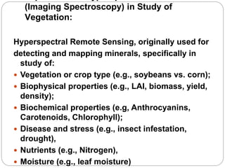
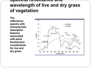
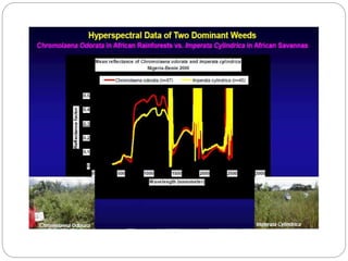
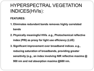
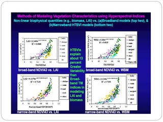
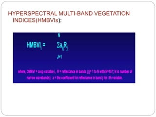
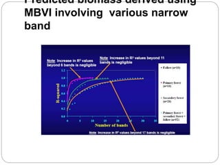
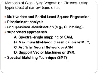
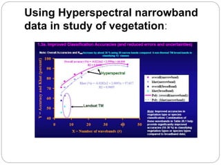
HYPERSPECTRAL REMOTE
SENSING OF VEGETATION
HYPERSPECTRAL DATA
 It consists of hundreds or thousands of
narrow-wavebands (as narrow as 1; but
generally less than 5 nm) along the
electromagnetic spectrum;
 It is important to have narrowbands that are
contiguous for strict definition of
hyperspectral data;
 Hyperspectral Data is fast emerging to
provide practical solutions in characterizing,
quantifying, modeling, and mapping natural
vegetation and agricultural crops.
(Imaging Spectroscopy) in Study of
Vegetation:
Hyperspectral Remote Sensing, originally used for
detecting and mapping minerals, specifically in
study of:
 Vegetation or crop type (e.g., soybeans vs. corn);
 Biophysical properties (e.g., LAI, biomass, yield,
density);
 Biochemical properties (e.g, Anthrocyanins,
Carotenoids, Chlorophyll);
 Disease and stress (e.g., insect infestation,
drought),
 Nutrients (e.g., Nitrogen),
 Moisture (e.g., leaf moisture)
Spectral reflectance and
wavelength of live and dry grass
of vegetation
The
reflectance
spectra with
characteristic
absorption
features
associated
with plant
biochemical
constitutents
for live and
dry grass
HYPERSPECTRAL VEGETATION
INDICES(HVIs):
FEATURES:
1. Eliminates redundant bands removes highly correlated
bands
2. Physically meaningful HVIs .e.g., Photochemical reflective
index (PRI) as proxy for light use efficiency (LUE)
3. Significant improvement over broadband indices .e.g.,
reducing saturation of broadbands, providing greater
sensitivity (e.g., an index involving NIR reflective maxima @
900 nm and red absorption maxima @680 nm.
METHOD FOR MODELLING
VEGETATION CHARACTERISTICS
USING HYPERSPECTRAL INDICES
 Hyperspectral Two-band Vegetation Indices
(TBVIs) = 12246 unique indices for 157 useful
Hyperion bands of data.
HYPERION:
 acquired over 400-2500 nm in 220 narrow-bands
each of 10-nm wide bands. Of these there are 196
bands that are calibrated. These are: (i) bands 8
(427.55 nm) to 57 (925.85 nm) in the visible and
near-infrared; and (ii) bands 79 (932.72 nm) to
band 224 (2395.53 nm) in the short wave infrared.
 However, there was significant noise in the data over the
1206–1437 nm, 1790– 1992 nm, and 2365–2396 nm spectral
ranges. When the Hyperion bands in this region were
dropped, 157 useful bands remained.
 Spectroradiometer:
acquired over 400-2500 nm in 2100 narrow-bands each of 1-
nm wide. However, 1-nm wide data were aggregated to 10-
nm wide to coincide with Hyperion bands.
However, there was significant noise in the data over the
1350-1440 nm, 1790-1990 nm, and 2360-2500 nm spectral
ranges was seriously affected by atmospheric absorption
and noise. The remaining good noise free data were in 400-
1350 nm, and 1440-1790 nm, 1990-2360 nm.
HYPERSPECTRAL MULTI-BAND VEGETATION
INDICES(HMBVIs):
Predicted biomass derived using
MBVI involving various narrow
band
Methods of Classifying Vegetation Classes using
hyperspectral narrow band data:
 Multivariate and Partial Least Square Regression.
 Discriminant analysis
 unsupervised classification (e.g., Clustering).
 supervised approaches
A. Spectral-angle mapping or SAM,
B. Maximum likelihood classification or MLC,
C. Artificial Neural Network or ANN,
D. Support Vector Machines or SVM.
 Spectral Matching Technique (SMT)
Using Hyperspectral narrowband
data in study of vegetation:
APPLICATIONS:
 Hyperspectral remote sensing studies have
shown a variety of applications including varietal
discrimination, moisture stress, parameter
retrieval, pest and diseases assessment,etc.
 A large part of hyperspectral data may be
redundant in agricultural application studies.
 It is important to identify and remove the
redundant bands from further analysis to ensure
most effective and efficient use of hyperspectral
data in agriculture. However, some of the
redundant bands in one application may be useful
in some other application and this must be taken
into consideration while data mining methods are
used.
THANK YOU….

Hyperspectral remote sensing of vegetation

  • 1.
  • 2.
    HYPERSPECTRAL DATA  Itconsists of hundreds or thousands of narrow-wavebands (as narrow as 1; but generally less than 5 nm) along the electromagnetic spectrum;  It is important to have narrowbands that are contiguous for strict definition of hyperspectral data;  Hyperspectral Data is fast emerging to provide practical solutions in characterizing, quantifying, modeling, and mapping natural vegetation and agricultural crops.
  • 3.
    (Imaging Spectroscopy) inStudy of Vegetation: Hyperspectral Remote Sensing, originally used for detecting and mapping minerals, specifically in study of:  Vegetation or crop type (e.g., soybeans vs. corn);  Biophysical properties (e.g., LAI, biomass, yield, density);  Biochemical properties (e.g, Anthrocyanins, Carotenoids, Chlorophyll);  Disease and stress (e.g., insect infestation, drought),  Nutrients (e.g., Nitrogen),  Moisture (e.g., leaf moisture)
  • 4.
    Spectral reflectance and wavelengthof live and dry grass of vegetation The reflectance spectra with characteristic absorption features associated with plant biochemical constitutents for live and dry grass
  • 6.
    HYPERSPECTRAL VEGETATION INDICES(HVIs): FEATURES: 1. Eliminatesredundant bands removes highly correlated bands 2. Physically meaningful HVIs .e.g., Photochemical reflective index (PRI) as proxy for light use efficiency (LUE) 3. Significant improvement over broadband indices .e.g., reducing saturation of broadbands, providing greater sensitivity (e.g., an index involving NIR reflective maxima @ 900 nm and red absorption maxima @680 nm.
  • 7.
    METHOD FOR MODELLING VEGETATIONCHARACTERISTICS USING HYPERSPECTRAL INDICES  Hyperspectral Two-band Vegetation Indices (TBVIs) = 12246 unique indices for 157 useful Hyperion bands of data. HYPERION:  acquired over 400-2500 nm in 220 narrow-bands each of 10-nm wide bands. Of these there are 196 bands that are calibrated. These are: (i) bands 8 (427.55 nm) to 57 (925.85 nm) in the visible and near-infrared; and (ii) bands 79 (932.72 nm) to band 224 (2395.53 nm) in the short wave infrared.
  • 8.
     However, therewas significant noise in the data over the 1206–1437 nm, 1790– 1992 nm, and 2365–2396 nm spectral ranges. When the Hyperion bands in this region were dropped, 157 useful bands remained.  Spectroradiometer: acquired over 400-2500 nm in 2100 narrow-bands each of 1- nm wide. However, 1-nm wide data were aggregated to 10- nm wide to coincide with Hyperion bands. However, there was significant noise in the data over the 1350-1440 nm, 1790-1990 nm, and 2360-2500 nm spectral ranges was seriously affected by atmospheric absorption and noise. The remaining good noise free data were in 400- 1350 nm, and 1440-1790 nm, 1990-2360 nm.
  • 10.
  • 11.
    Predicted biomass derivedusing MBVI involving various narrow band
  • 12.
    Methods of ClassifyingVegetation Classes using hyperspectral narrow band data:  Multivariate and Partial Least Square Regression.  Discriminant analysis  unsupervised classification (e.g., Clustering).  supervised approaches A. Spectral-angle mapping or SAM, B. Maximum likelihood classification or MLC, C. Artificial Neural Network or ANN, D. Support Vector Machines or SVM.  Spectral Matching Technique (SMT)
  • 13.
    Using Hyperspectral narrowband datain study of vegetation:
  • 14.
    APPLICATIONS:  Hyperspectral remotesensing studies have shown a variety of applications including varietal discrimination, moisture stress, parameter retrieval, pest and diseases assessment,etc.  A large part of hyperspectral data may be redundant in agricultural application studies.  It is important to identify and remove the redundant bands from further analysis to ensure most effective and efficient use of hyperspectral data in agriculture. However, some of the redundant bands in one application may be useful in some other application and this must be taken into consideration while data mining methods are used.
  • 15.