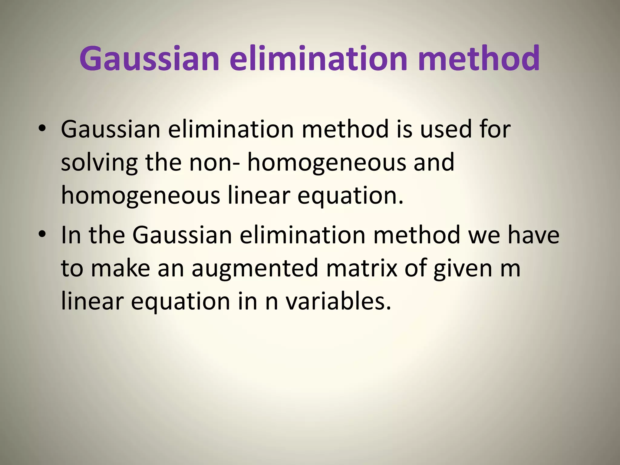
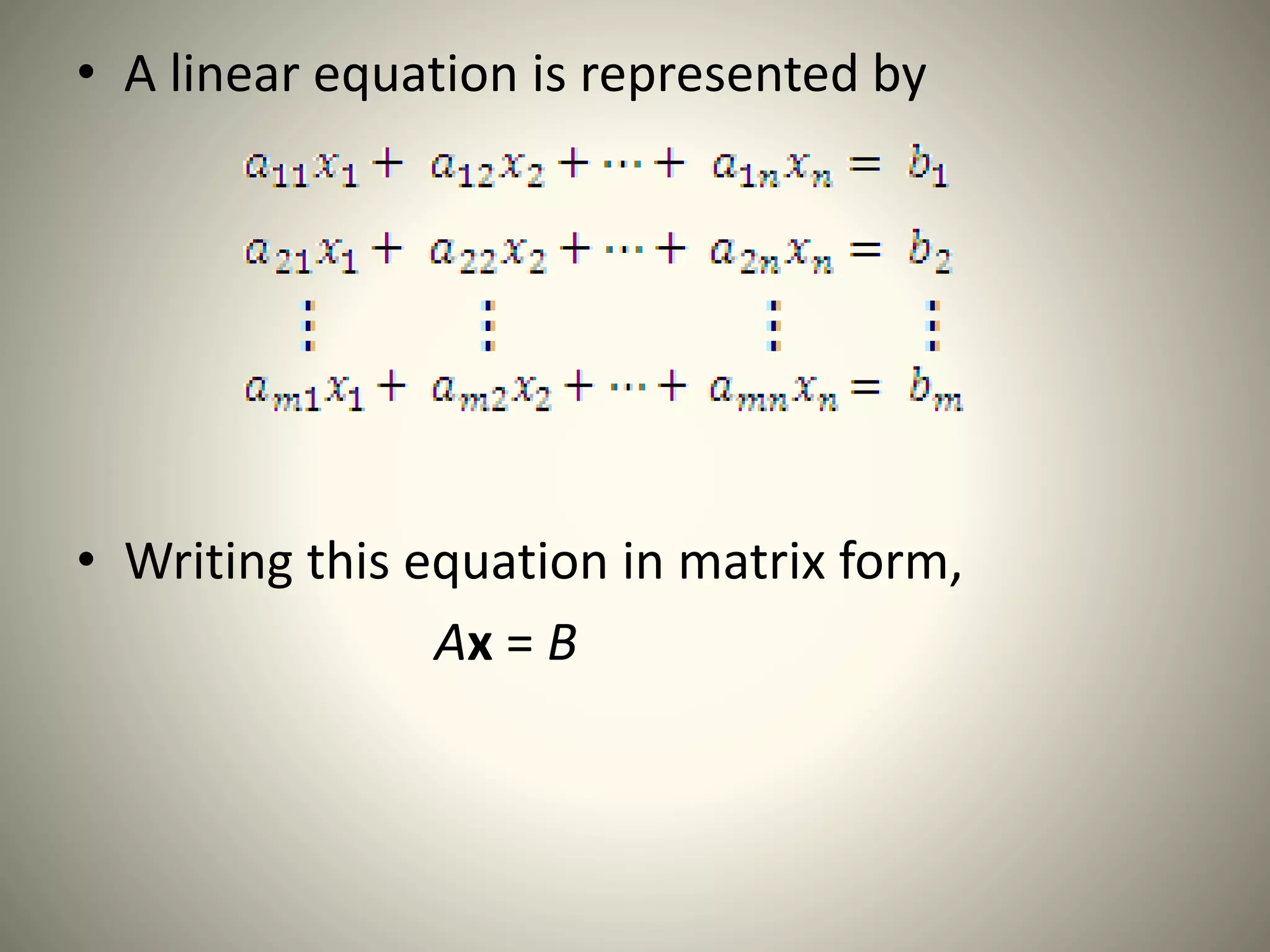
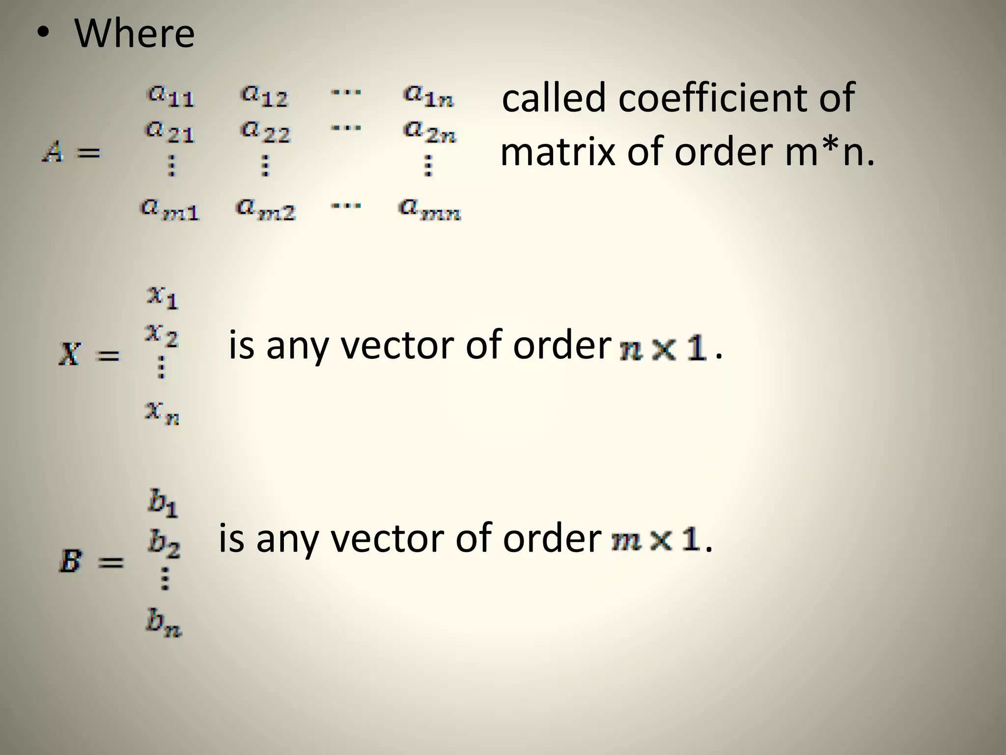
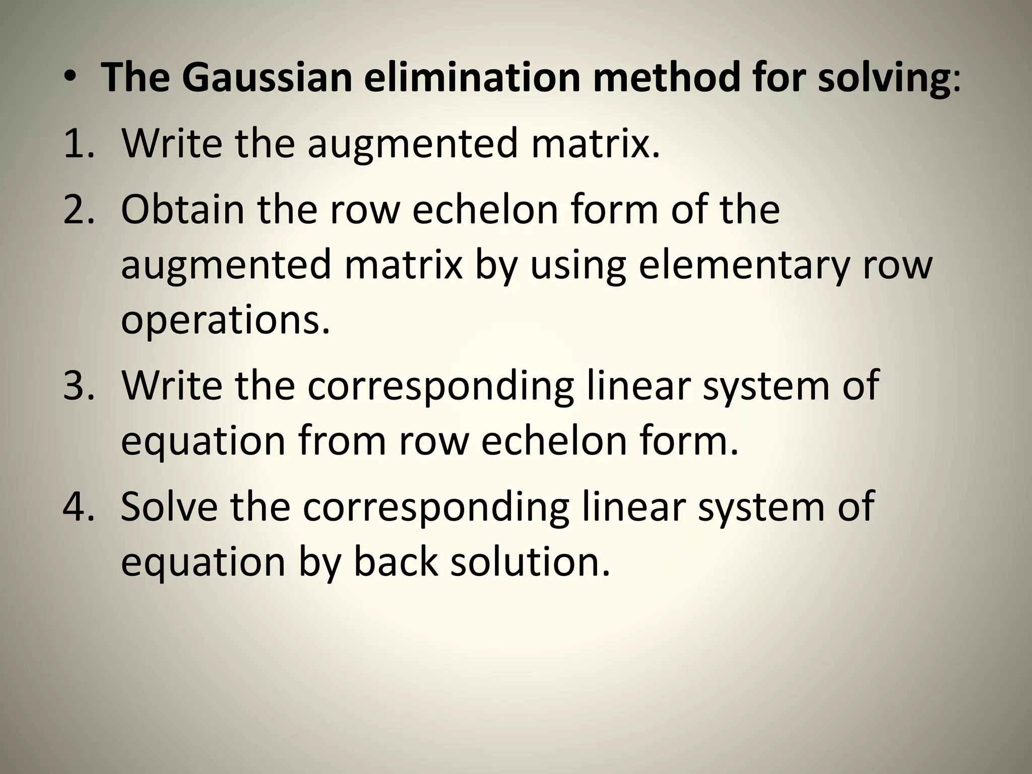
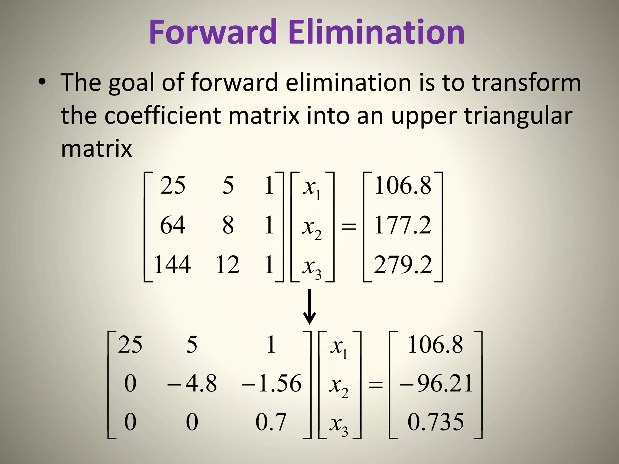
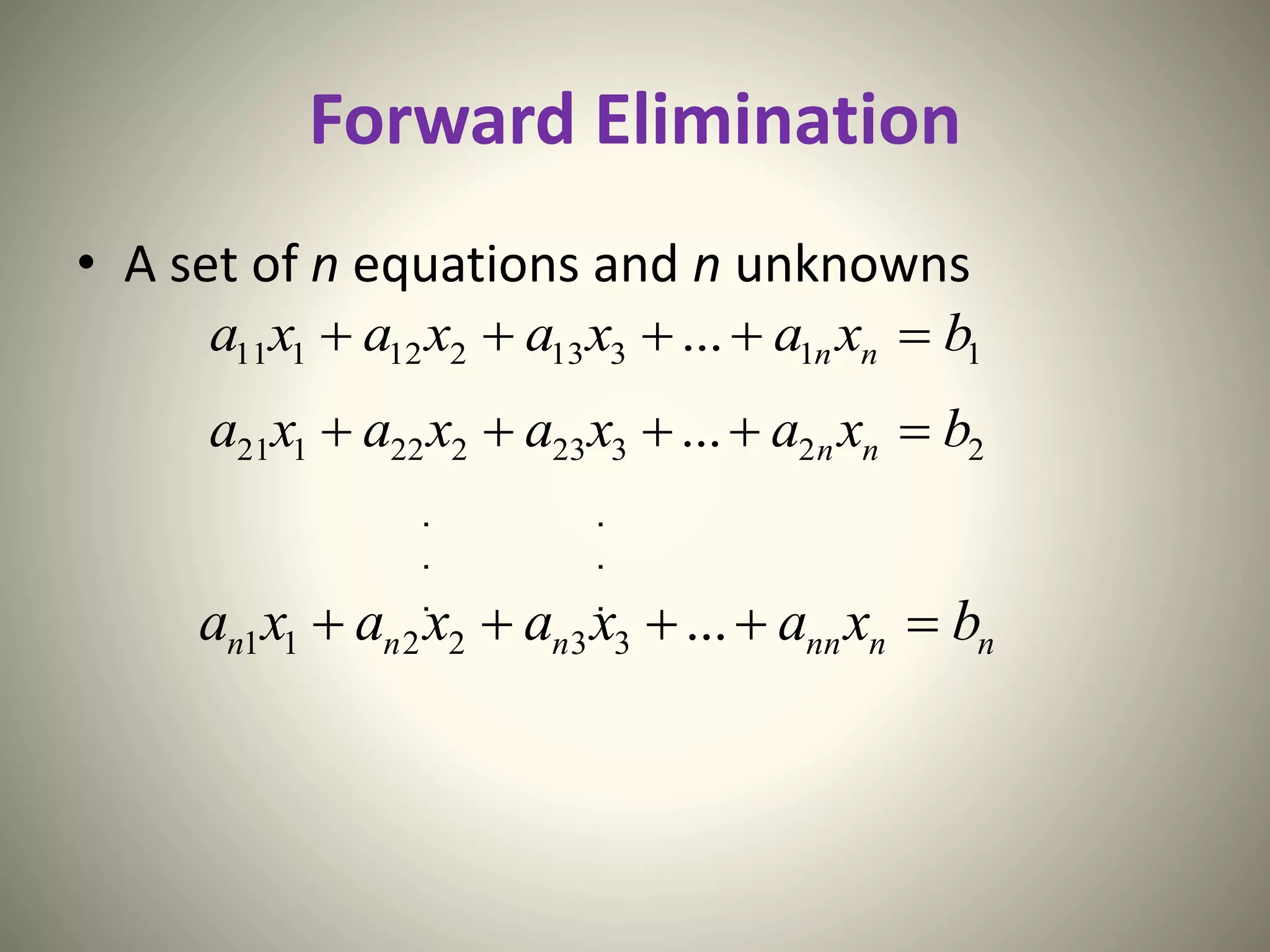
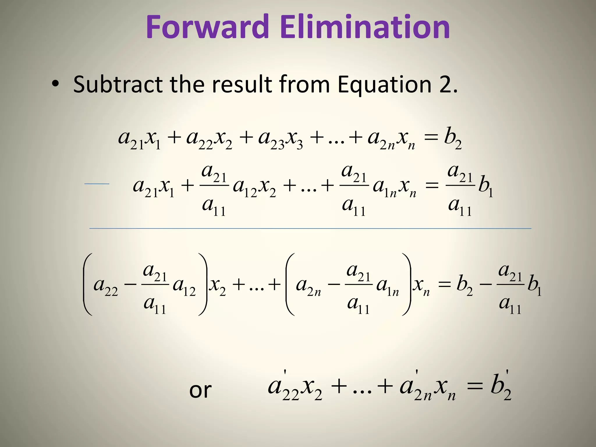
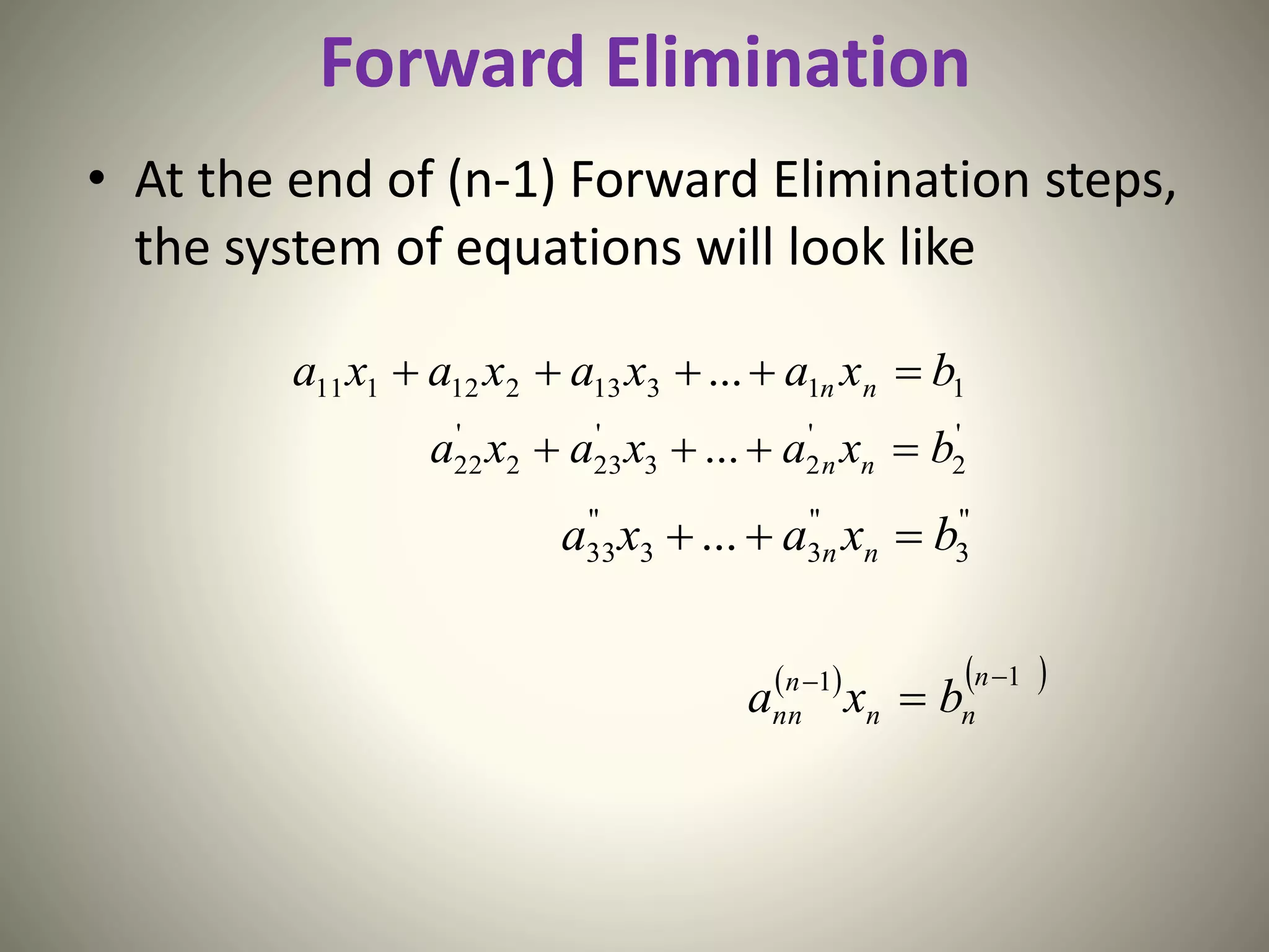
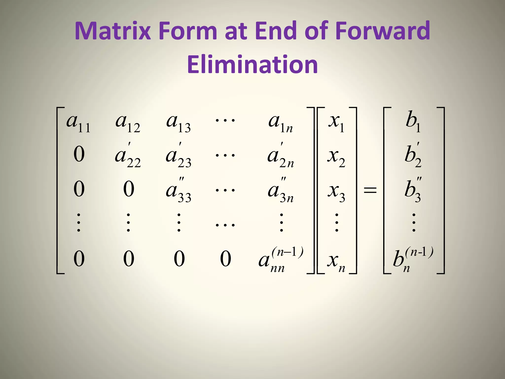
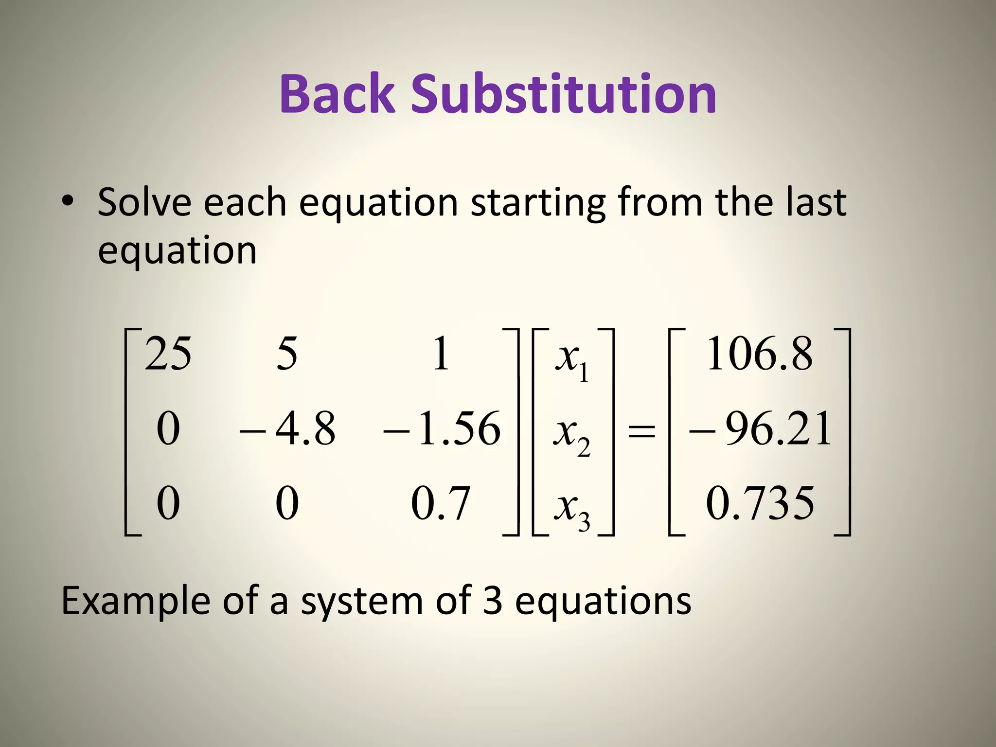
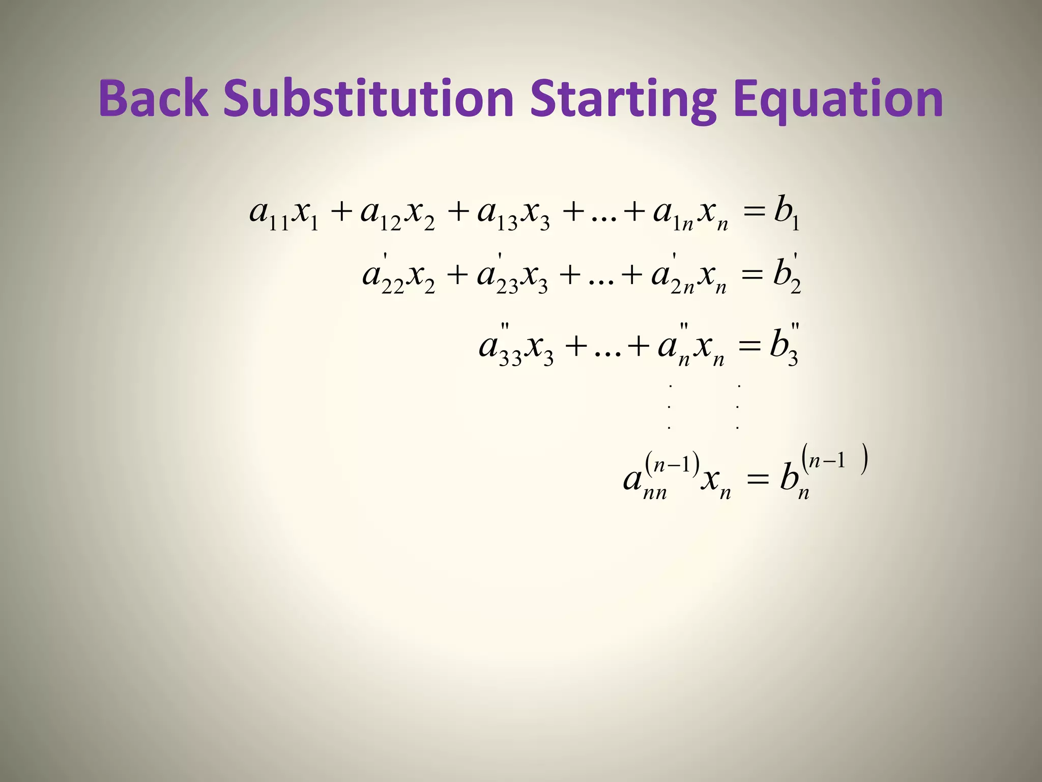
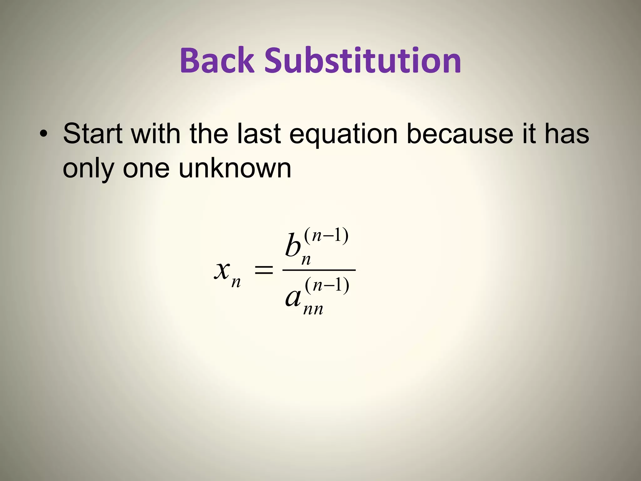
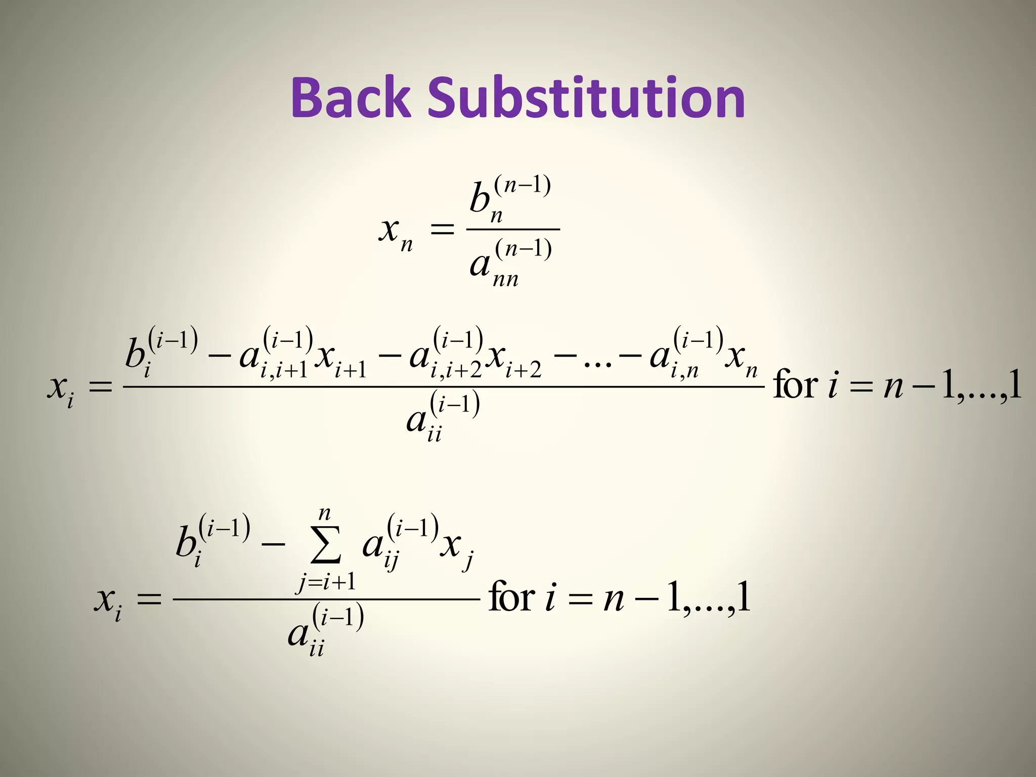
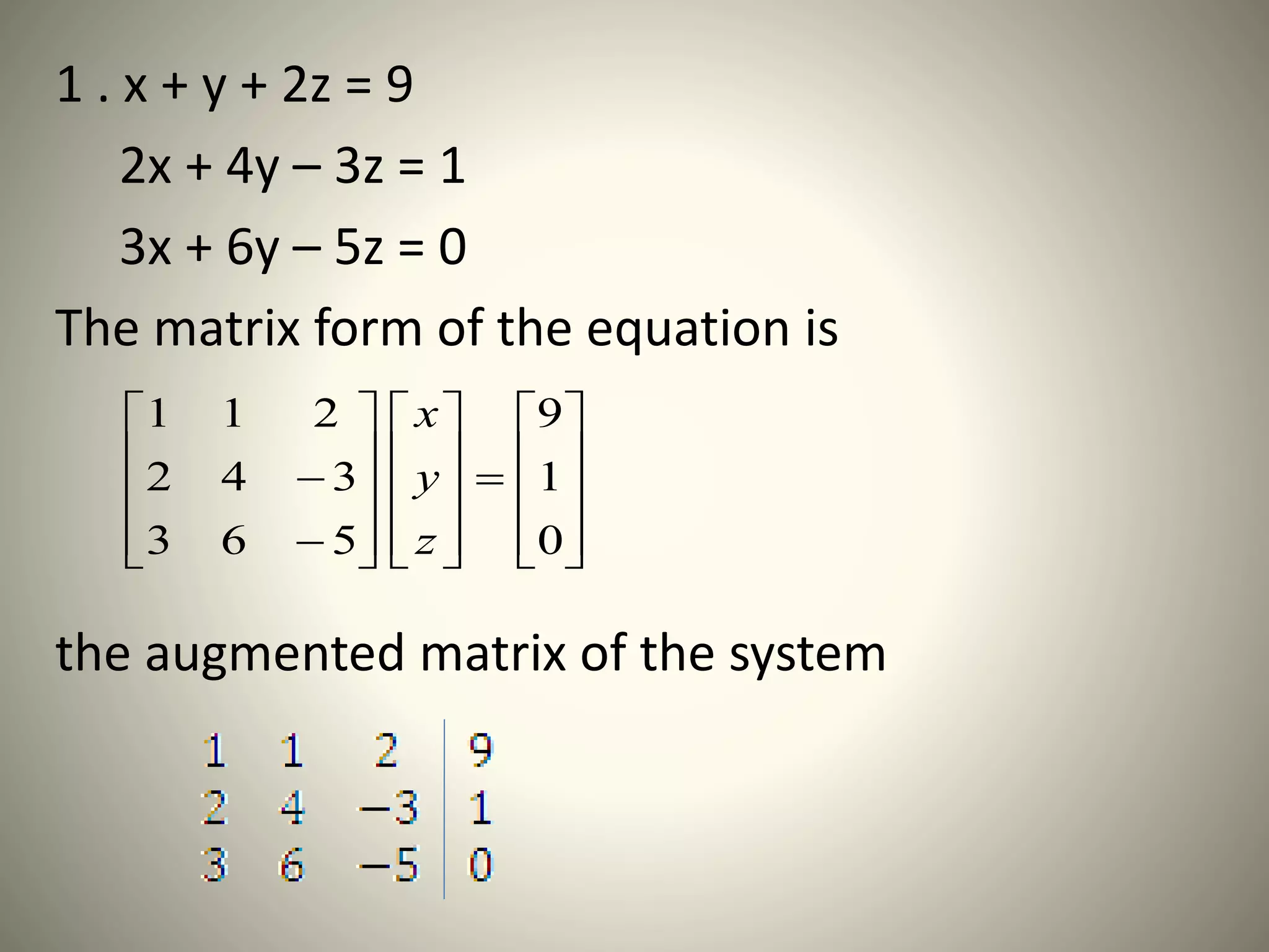
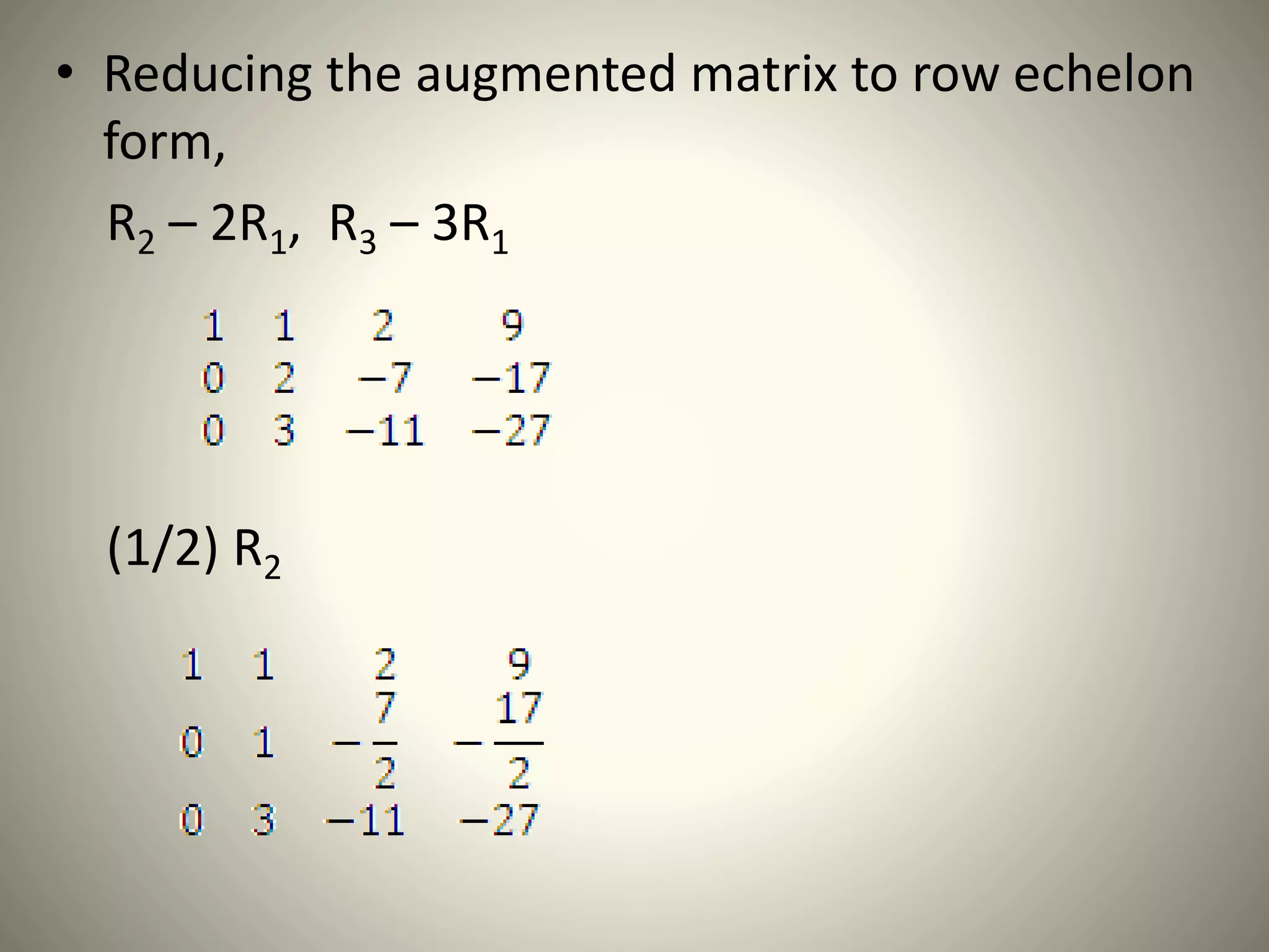
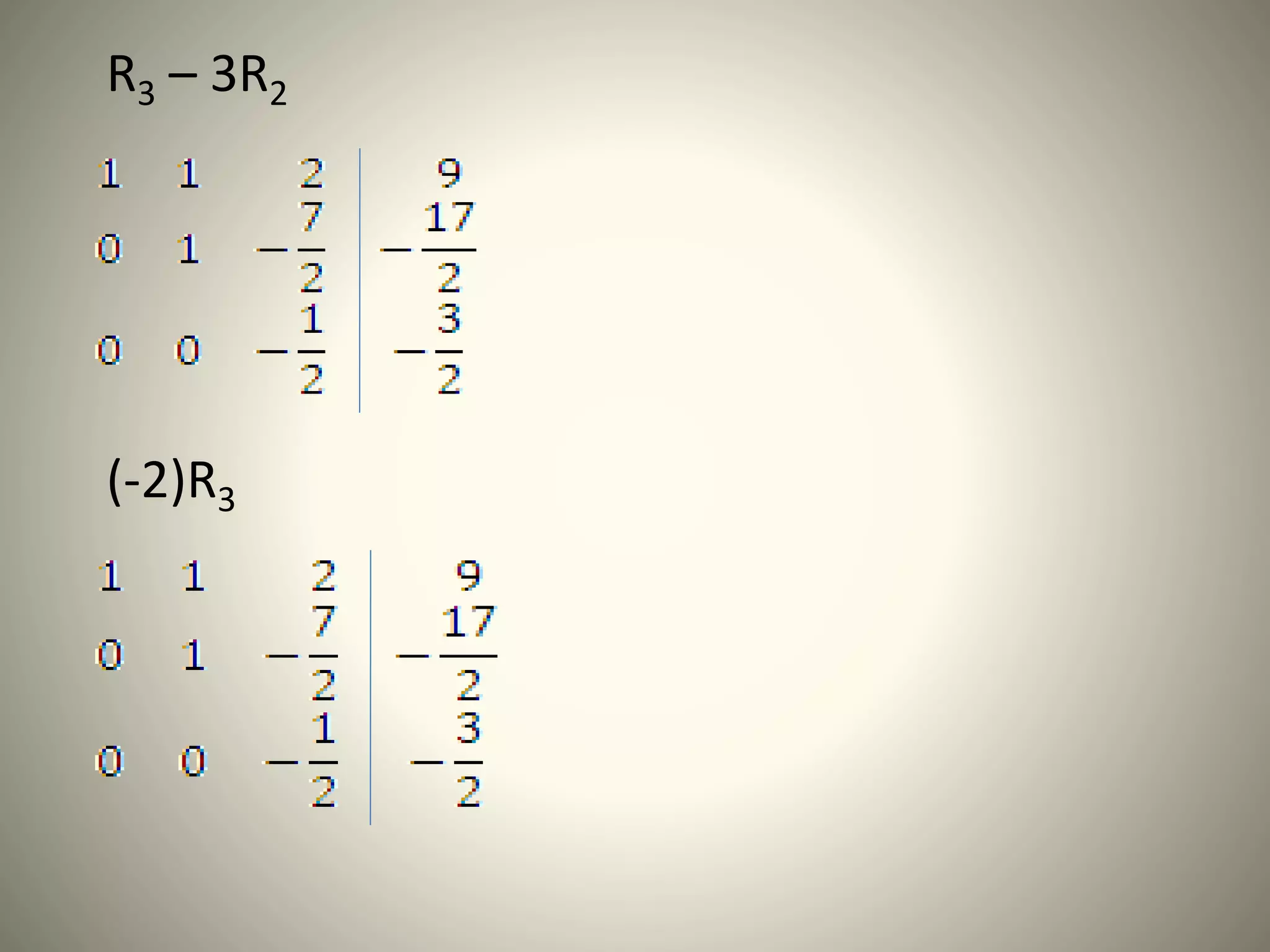
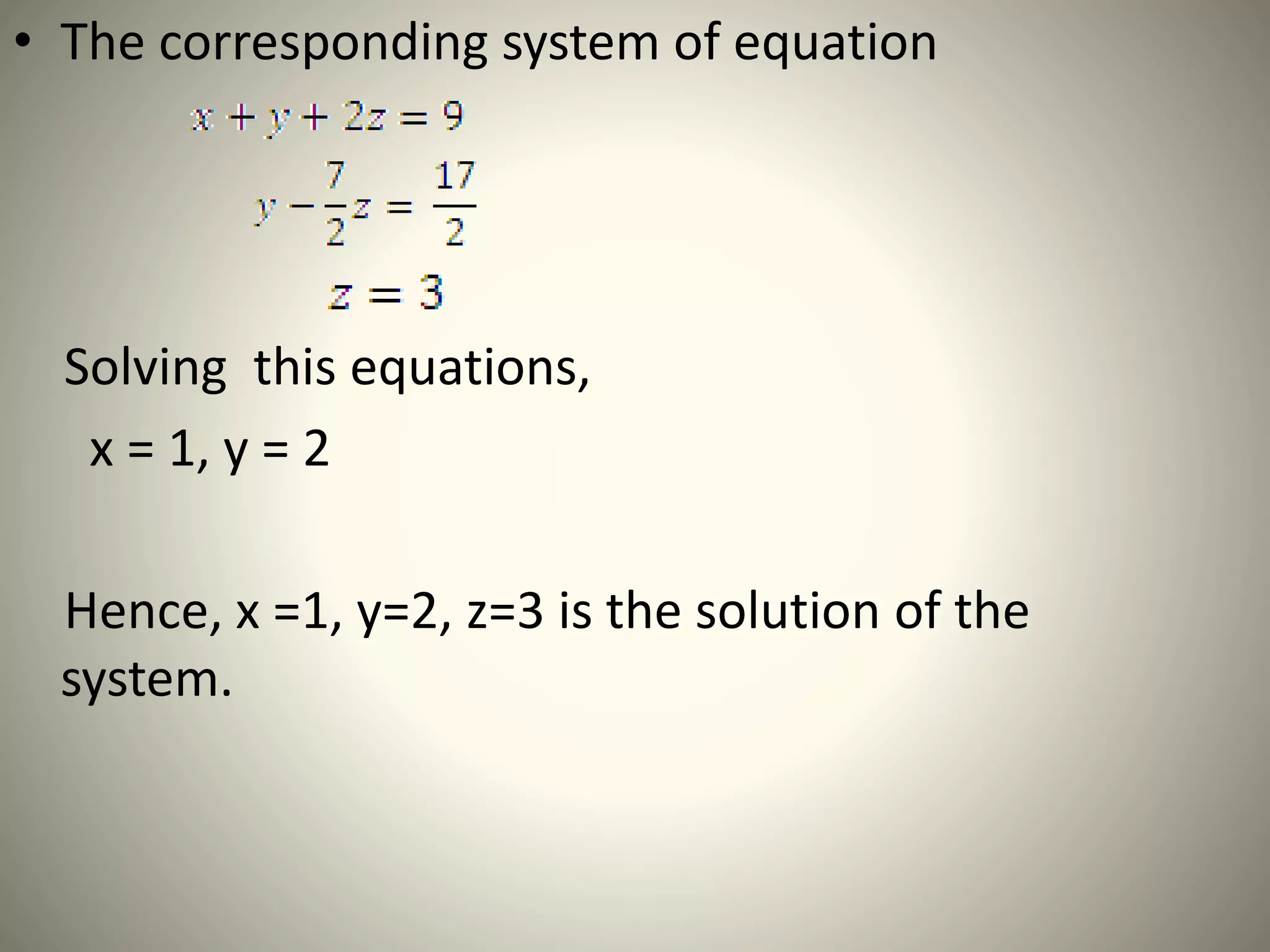
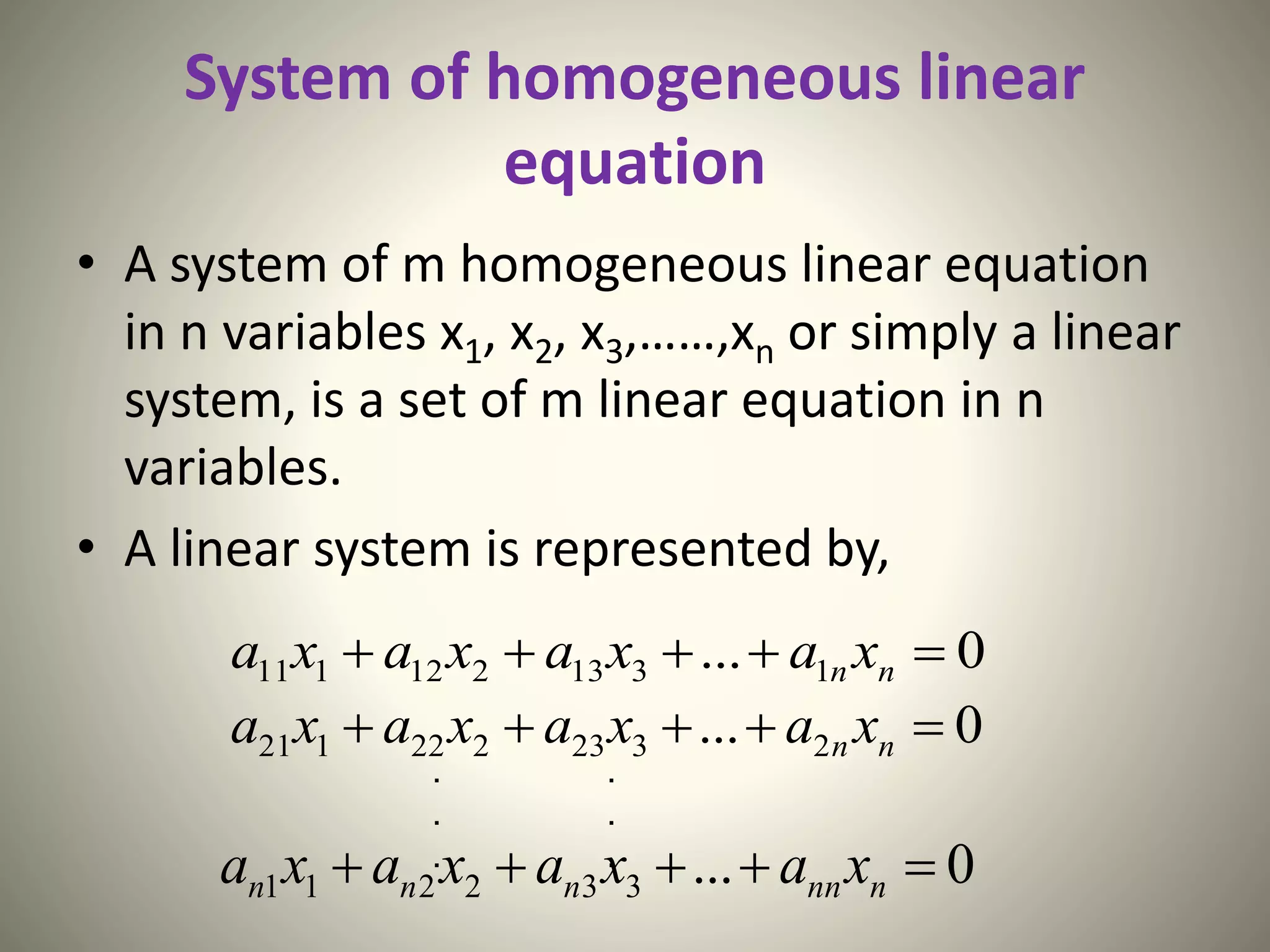
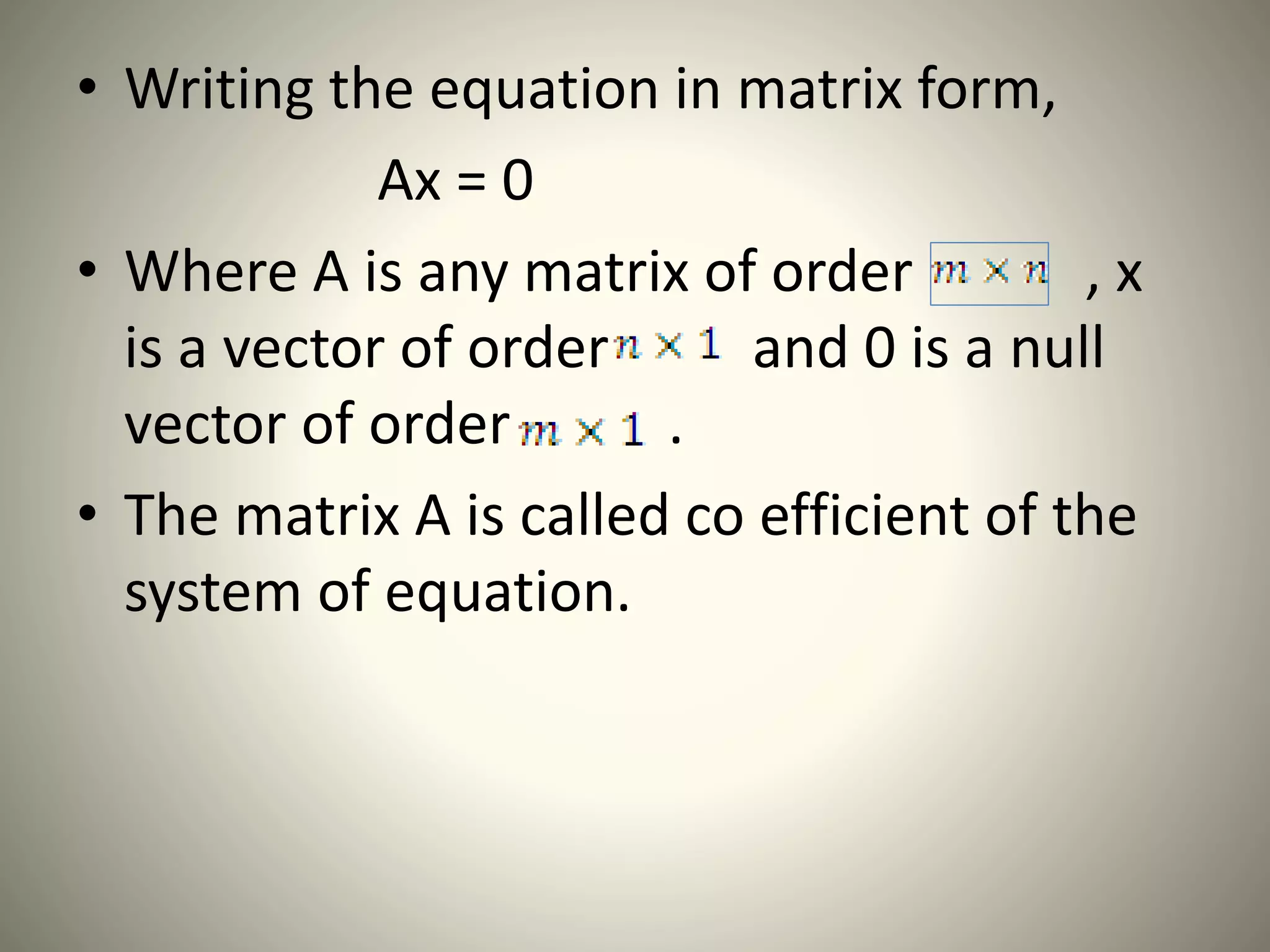
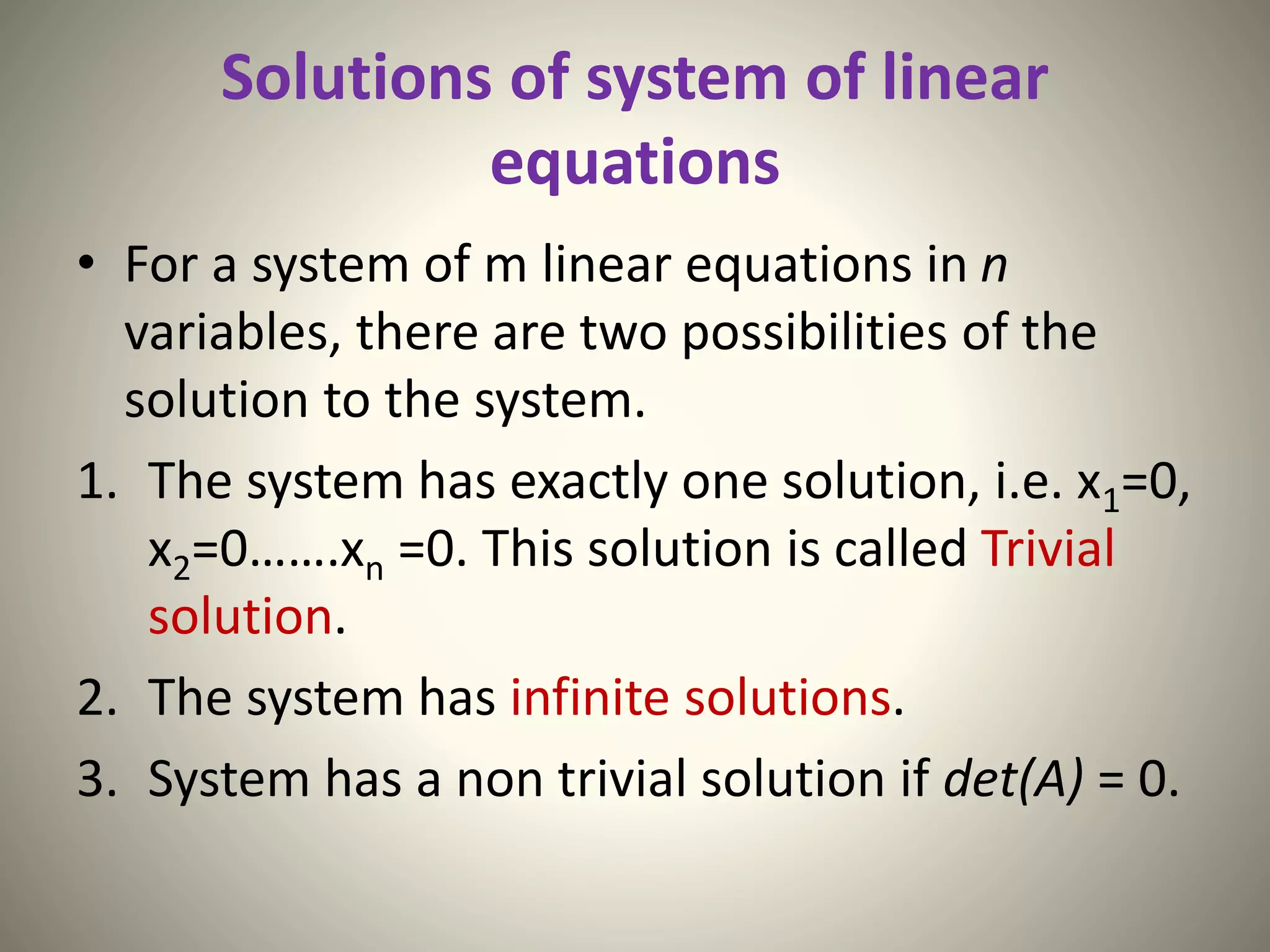
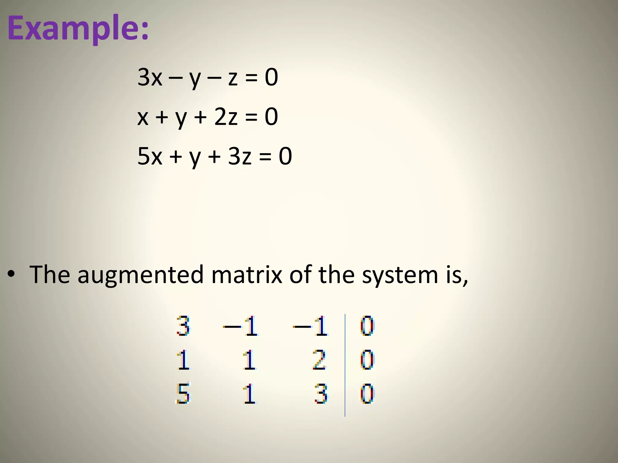
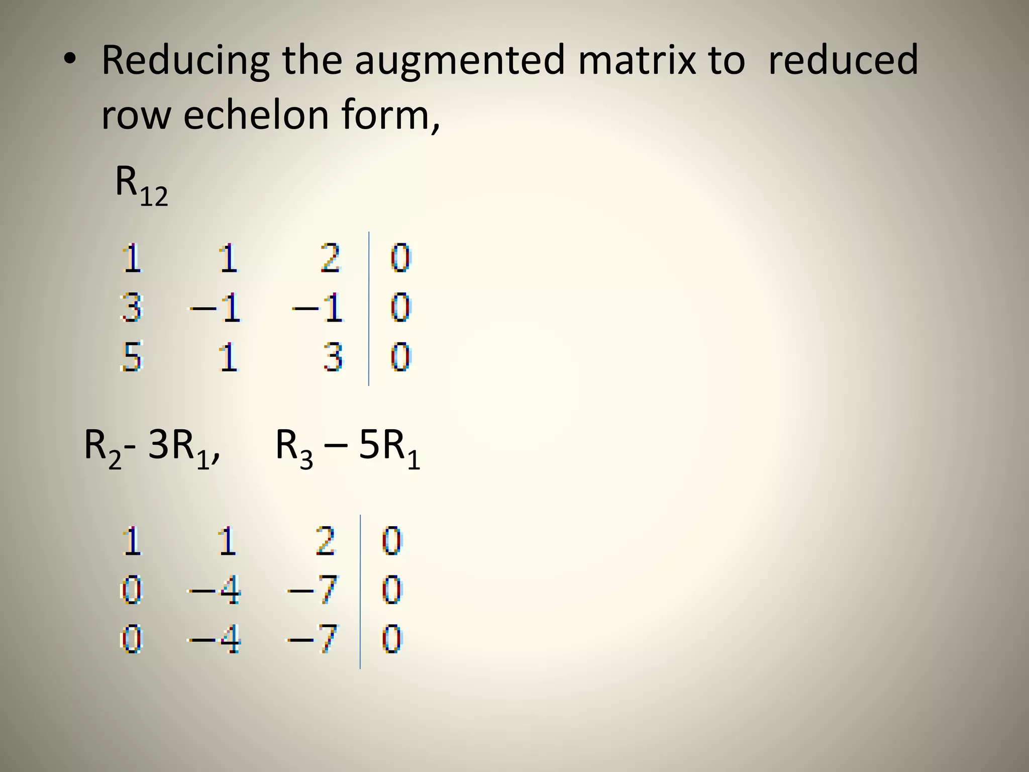
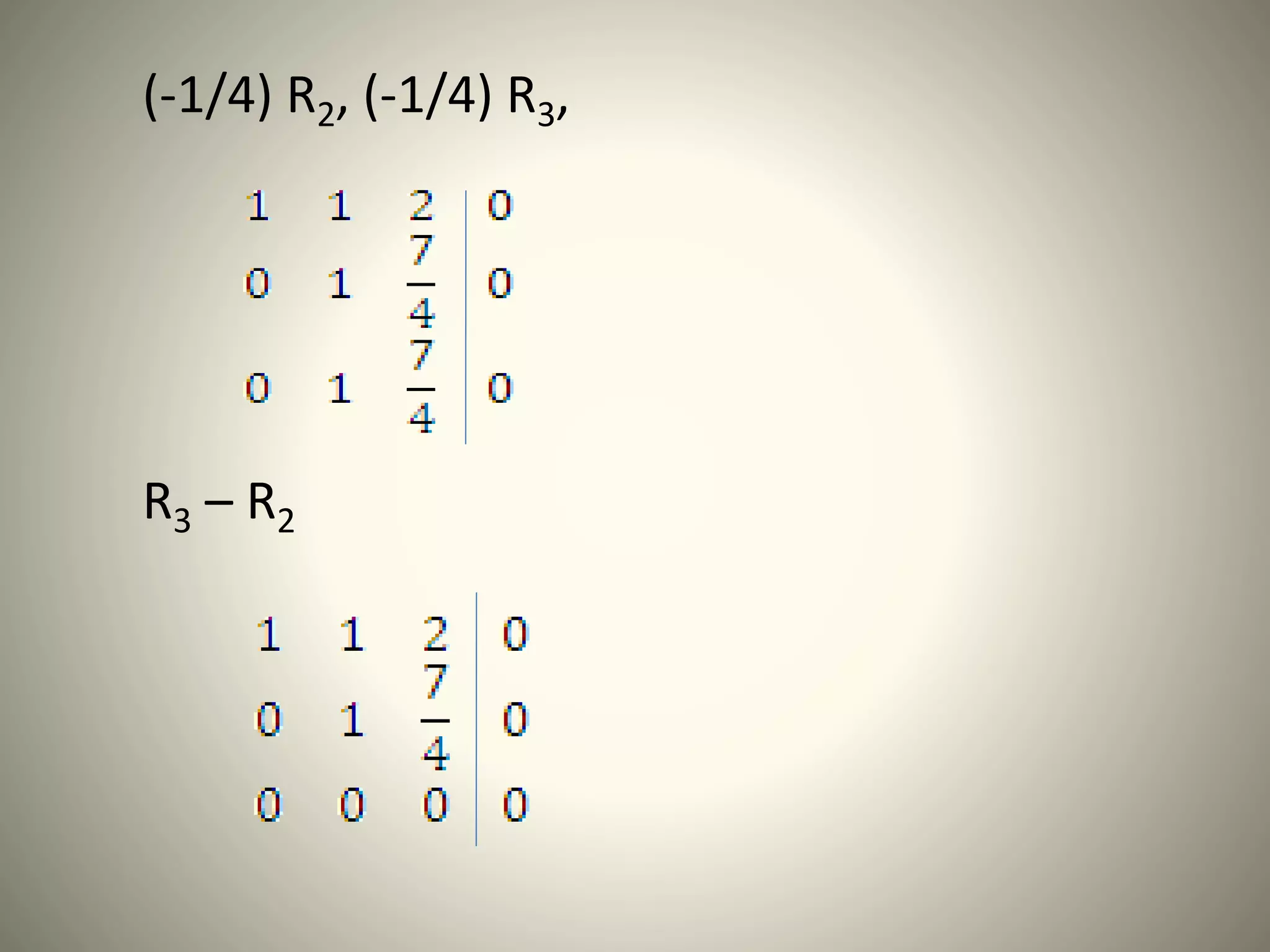
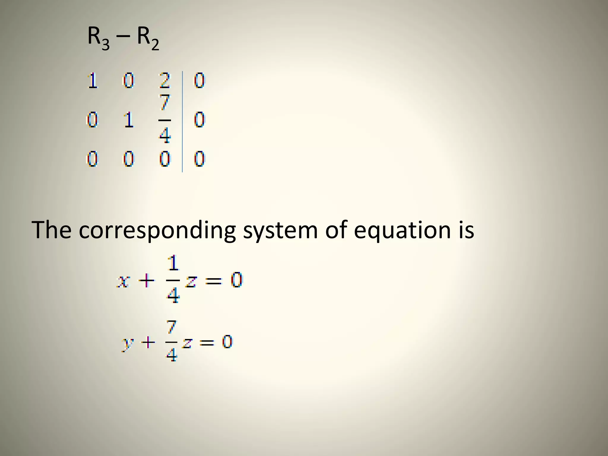
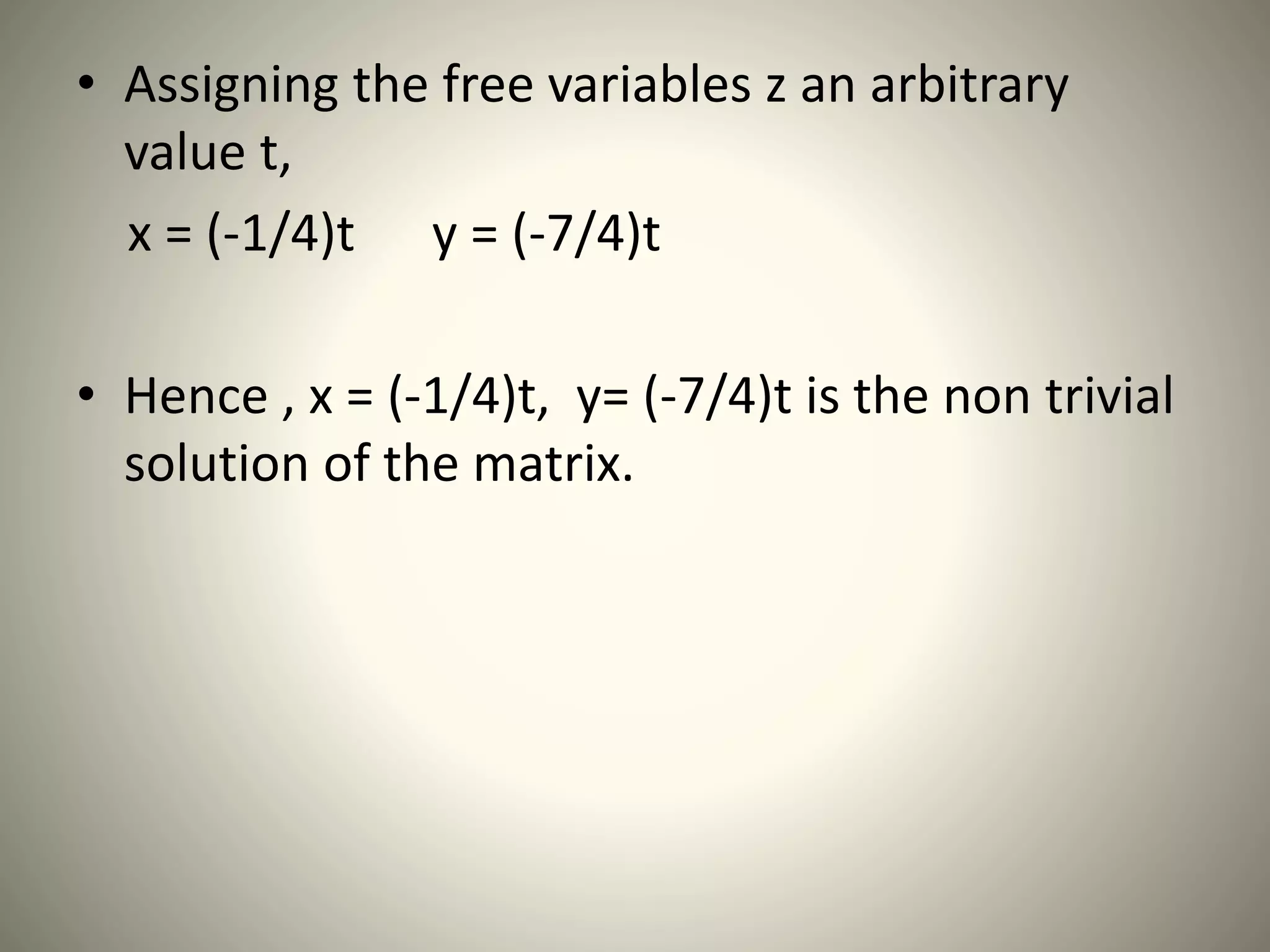
Gaussian Elimination Method &
Homogeneous Linear Equation
Prepared By:
130110120007 – Ravi
130110120008 – Hemdeep Bhavsar
130110120009 – Nayan Chauhan
130110120010 – Chintan Katerecha
130110120011 – Chitt Kakadiya
130110120012 – Yashraj Chudasama
Faculty :-
VRS Sir
Gaussian elimination method
• Gaussian elimination method is used for
solving the non- homogeneous and
homogeneous linear equation.
• In the Gaussian elimination method we have
to make an augmented matrix of given m
linear equation in n variables.
• A system of m homogeneous or non
homogeneous linear equations in n
variables x1, x2, …,xn or simply a
linear system is a set of m linear
equation, each in n variables.
• A linear equation is represented by
• Writing this equation in matrix form,
Ax = B
• Where
called coefficient of
matrix of order m*n.
is any vector of order .
• To solve a system of linear equation,
elementary transformation are used to
reduce the augmented matrix to either
row echelon form or reduced row echelon
form.
• Reducing the augmented matrix to row
echelon form is called Gaussian elimination
method.
• The Gaussian elimination method for solving:
1. Write the augmented matrix.
2. Obtain the row echelon form of the
augmented matrix by using elementary row
operations.
3. Write the corresponding linear system of
equation from row echelon form.
4. Solve the corresponding linear system of
equation by back solution.
Forward Elimination
• The goal of forward elimination is to transform
the coefficient matrix into an upper triangular
matrix































2.279
2.177
8.106
112144
1864
1525
3
2
1
x
x
x
































735.0
21.96
8.106
7.000
56.18.40
1525
3
2
1
x
x
x
Forward Elimination
• A set of n equations and n unknowns
11313212111 ... bxaxaxaxa nn 
22323222121 ... bxaxaxaxa nn 
. .
. .
. .
nnnnnnn bxaxaxaxa  ...332211
Forward Elimination
• Subtract the result from Equation 2.
or
22323222121 ... bxaxaxaxa nn 
1
11
21
1
11
21
212
11
21
121 ... b
a
a
xa
a
a
xa
a
a
xa nn 
1
11
21
21
11
21
2212
11
21
22 ... b
a
a
bxa
a
a
axa
a
a
a nnn 












'
2
'
22
'
22 ... bxaxa nn 
Forward Elimination
• At the end of (n-1) Forward Elimination steps,
the system of equations will look like
11313212111 ... bxaxaxaxa nn 
'
2
'
23
'
232
'
22 ... bxaxaxa nn 
"
3
"
33
"
33 ... bxaxa nn 
   11 

n
nn
n
nn bxa
Matrix Form at End of Forward
Elimination

















































 )(n-
n
"
'
n
)(n
nn
"
n
"
'
n
''
n
b
b
b
b
x
x
x
x
a
aa
aaa
aaaa
1
3
2
1
3
2
1
1
333
22322
1131211
0000
00
0




Back Substitution
• Solve each equation starting from the last
equation
Example of a system of 3 equations
































735.0
21.96
8.106
7.000
56.18.40
1525
3
2
1
x
x
x
Back Substitution Starting Equation
11313212111 ... bxaxaxaxa nn 
'
2
'
23
'
232
'
22 ... bxaxaxa nn 
"
3
"
3
"
33 ... bxaxa nn 
. .
. .
. .
   11 

n
nn
n
nn bxa
Back Substitution
• Start with the last equation because it has
only one unknown
)1(
)1(


 n
nn
n
n
n
a
b
x
Back Substitution
)1(
)1(


 n
nn
n
n
n
a
b
x
       
  1,...,1for
...
1
1
,2
1
2,1
1
1,
1


 







ni
a
xaxaxab
x i
ii
n
i
nii
i
iii
i
ii
i
i
i
   
  1,...,1for1
1
11


 


ni
a
xab
x i
ii
n
ij
j
i
ij
i
i
i
1 . x + y + 2z = 9
2x + 4y – 3z = 1
3x + 6y – 5z = 0
The matrix form of the equation is
the augmented matrix of the system

































0
1
9
563
342
211
z
y
x
• Reducing the augmented matrix to row echelon
form,
R2 – 2R1, R3 – 3R1
(1/2) R2
R3 – 3R2
(-2)R3
• The corresponding system of equation
Solving this equations,
x = 1, y = 2
Hence, x =1, y=2, z=3 is the solution of the
system.
System of homogeneous linear
equation
• A system of m homogeneous linear equation
in n variables x1, x2, x3,……,xn or simply a linear
system, is a set of m linear equation in n
variables.
• A linear system is represented by,
0... 1313212111  nn xaxaxaxa
0... 2323222121  nn xaxaxaxa
0...332211  nnnnnn xaxaxaxa
. .
. .
. .
• Writing the equation in matrix form,
Ax = 0
• Where A is any matrix of order , x
is a vector of order and 0 is a null
vector of order .
• The matrix A is called co efficient of the
system of equation.
Solutions of system of linear
equations
• For a system of m linear equations in n
variables, there are two possibilities of the
solution to the system.
1. The system has exactly one solution, i.e. x1=0,
x2=0…….xn =0. This solution is called Trivial
solution.
2. The system has infinite solutions.
3. System has a non trivial solution if det(A) = 0.
Example:
3x – y – z = 0
x + y + 2z = 0
5x + y + 3z = 0
• The augmented matrix of the system is,
• Reducing the augmented matrix to reduced
row echelon form,
R12
R2- 3R1, R3 – 5R1
(-1/4) R2, (-1/4) R3,
R3 – R2
R3 – R2
The corresponding system of equation is
• Assigning the free variables z an arbitrary
value t,
x = (-1/4)t y = (-7/4)t
• Hence , x = (-1/4)t, y= (-7/4)t is the non trivial
solution of the matrix.

Gaussian elimination method & homogeneous linear equation

  • 1.
    Gaussian Elimination Method& Homogeneous Linear Equation Prepared By: 130110120007 – Ravi 130110120008 – Hemdeep Bhavsar 130110120009 – Nayan Chauhan 130110120010 – Chintan Katerecha 130110120011 – Chitt Kakadiya 130110120012 – Yashraj Chudasama Faculty :- VRS Sir
  • 2.
    Gaussian elimination method •Gaussian elimination method is used for solving the non- homogeneous and homogeneous linear equation. • In the Gaussian elimination method we have to make an augmented matrix of given m linear equation in n variables.
  • 3.
    • A systemof m homogeneous or non homogeneous linear equations in n variables x1, x2, …,xn or simply a linear system is a set of m linear equation, each in n variables.
  • 4.
    • A linearequation is represented by • Writing this equation in matrix form, Ax = B
  • 5.
    • Where called coefficientof matrix of order m*n. is any vector of order . is any vector of order .
  • 6.
    • To solvea system of linear equation, elementary transformation are used to reduce the augmented matrix to either row echelon form or reduced row echelon form. • Reducing the augmented matrix to row echelon form is called Gaussian elimination method.
  • 7.
    • The Gaussianelimination method for solving: 1. Write the augmented matrix. 2. Obtain the row echelon form of the augmented matrix by using elementary row operations. 3. Write the corresponding linear system of equation from row echelon form. 4. Solve the corresponding linear system of equation by back solution.
  • 8.
    Forward Elimination • Thegoal of forward elimination is to transform the coefficient matrix into an upper triangular matrix                                2.279 2.177 8.106 112144 1864 1525 3 2 1 x x x                                 735.0 21.96 8.106 7.000 56.18.40 1525 3 2 1 x x x
  • 9.
    Forward Elimination • Aset of n equations and n unknowns 11313212111 ... bxaxaxaxa nn  22323222121 ... bxaxaxaxa nn  . . . . . . nnnnnnn bxaxaxaxa  ...332211
  • 10.
    Forward Elimination • Subtractthe result from Equation 2. or 22323222121 ... bxaxaxaxa nn  1 11 21 1 11 21 212 11 21 121 ... b a a xa a a xa a a xa nn  1 11 21 21 11 21 2212 11 21 22 ... b a a bxa a a axa a a a nnn              ' 2 ' 22 ' 22 ... bxaxa nn 
  • 11.
    Forward Elimination • Atthe end of (n-1) Forward Elimination steps, the system of equations will look like 11313212111 ... bxaxaxaxa nn  ' 2 ' 23 ' 232 ' 22 ... bxaxaxa nn  " 3 " 33 " 33 ... bxaxa nn     11   n nn n nn bxa
  • 12.
    Matrix Form atEnd of Forward Elimination                                                   )(n- n " ' n )(n nn " n " ' n '' n b b b b x x x x a aa aaa aaaa 1 3 2 1 3 2 1 1 333 22322 1131211 0000 00 0    
  • 13.
    Back Substitution • Solveeach equation starting from the last equation Example of a system of 3 equations                                 735.0 21.96 8.106 7.000 56.18.40 1525 3 2 1 x x x
  • 14.
    Back Substitution StartingEquation 11313212111 ... bxaxaxaxa nn  ' 2 ' 23 ' 232 ' 22 ... bxaxaxa nn  " 3 " 3 " 33 ... bxaxa nn  . . . . . .    11   n nn n nn bxa
  • 15.
    Back Substitution • Startwith the last equation because it has only one unknown )1( )1(    n nn n n n a b x
  • 16.
    Back Substitution )1( )1(    n nn n n n a b x          1,...,1for ... 1 1 ,2 1 2,1 1 1, 1            ni a xaxaxab x i ii n i nii i iii i ii i i i       1,...,1for1 1 11       ni a xab x i ii n ij j i ij i i i
  • 17.
    1 . x+ y + 2z = 9 2x + 4y – 3z = 1 3x + 6y – 5z = 0 The matrix form of the equation is the augmented matrix of the system                                  0 1 9 563 342 211 z y x
  • 18.
    • Reducing theaugmented matrix to row echelon form, R2 – 2R1, R3 – 3R1 (1/2) R2
  • 19.
  • 20.
    • The correspondingsystem of equation Solving this equations, x = 1, y = 2 Hence, x =1, y=2, z=3 is the solution of the system.
  • 21.
    System of homogeneouslinear equation • A system of m homogeneous linear equation in n variables x1, x2, x3,……,xn or simply a linear system, is a set of m linear equation in n variables. • A linear system is represented by, 0... 1313212111  nn xaxaxaxa 0... 2323222121  nn xaxaxaxa 0...332211  nnnnnn xaxaxaxa . . . . . .
  • 22.
    • Writing theequation in matrix form, Ax = 0 • Where A is any matrix of order , x is a vector of order and 0 is a null vector of order . • The matrix A is called co efficient of the system of equation.
  • 23.
    Solutions of systemof linear equations • For a system of m linear equations in n variables, there are two possibilities of the solution to the system. 1. The system has exactly one solution, i.e. x1=0, x2=0…….xn =0. This solution is called Trivial solution. 2. The system has infinite solutions. 3. System has a non trivial solution if det(A) = 0.
  • 24.
    Example: 3x – y– z = 0 x + y + 2z = 0 5x + y + 3z = 0 • The augmented matrix of the system is,
  • 25.
    • Reducing theaugmented matrix to reduced row echelon form, R12 R2- 3R1, R3 – 5R1
  • 26.
    (-1/4) R2, (-1/4)R3, R3 – R2
  • 27.
    R3 – R2 Thecorresponding system of equation is
  • 28.
    • Assigning thefree variables z an arbitrary value t, x = (-1/4)t y = (-7/4)t • Hence , x = (-1/4)t, y= (-7/4)t is the non trivial solution of the matrix.