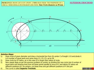
Download as PPSX, PPTX

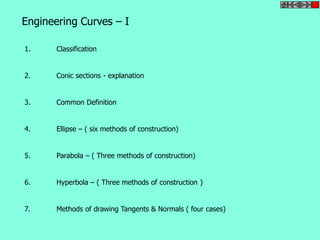
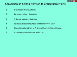
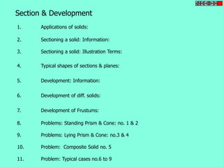
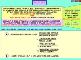
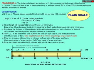
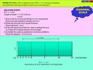
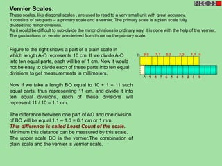
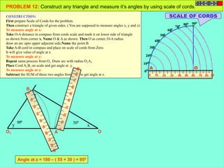
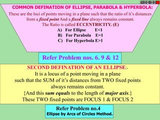
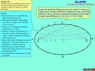
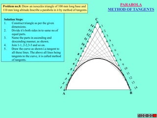
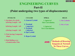
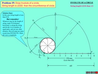
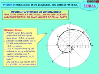
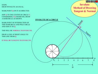
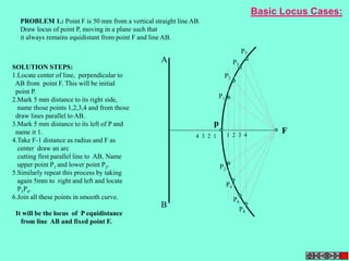
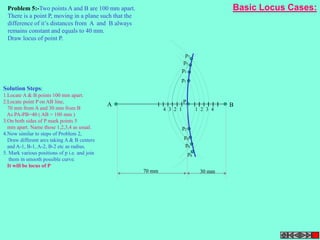
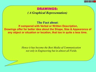
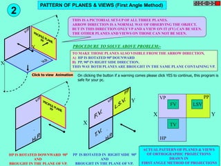
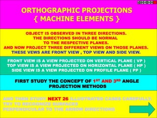
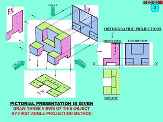
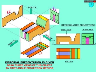
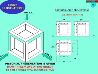
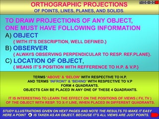
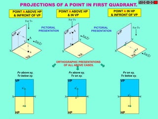
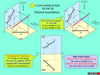
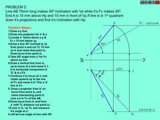
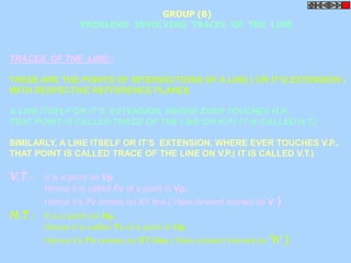
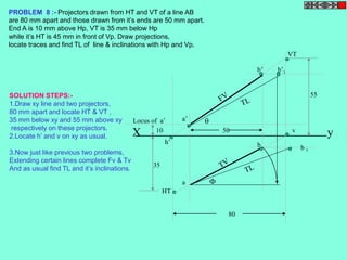
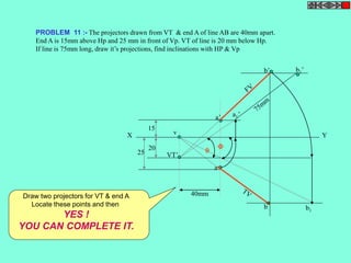
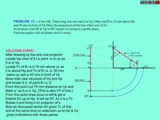
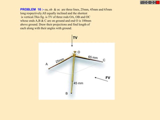
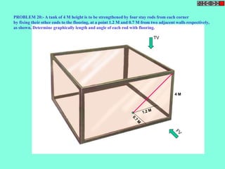
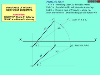
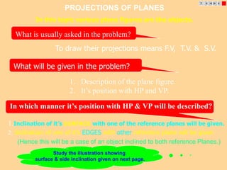
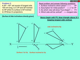
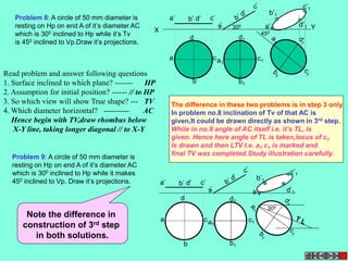
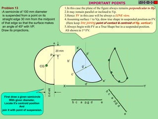
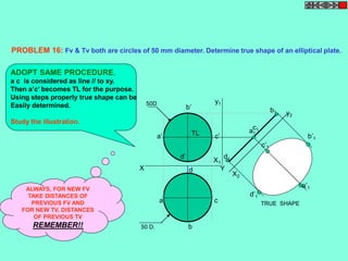
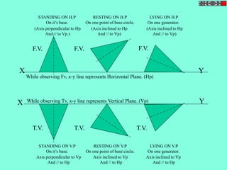
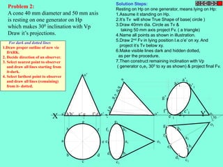
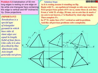
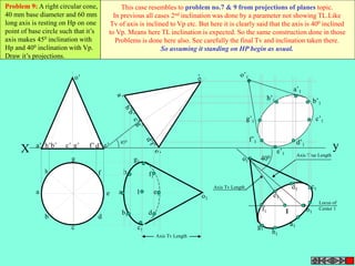
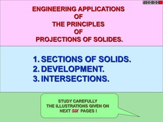
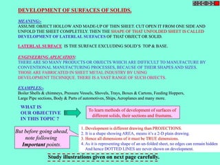
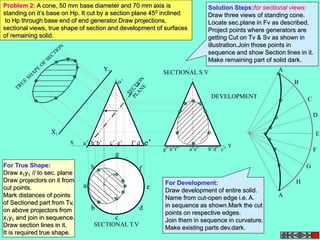
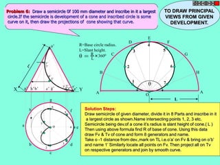
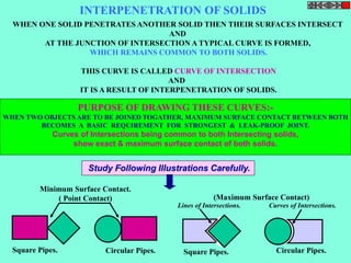
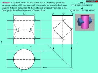
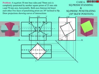
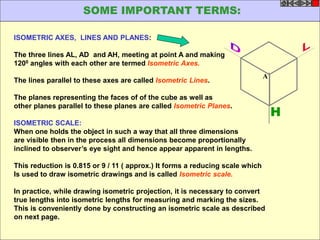
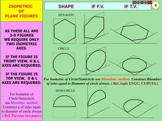
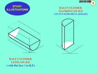
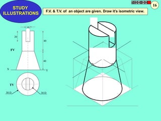
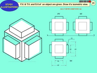
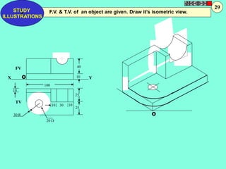
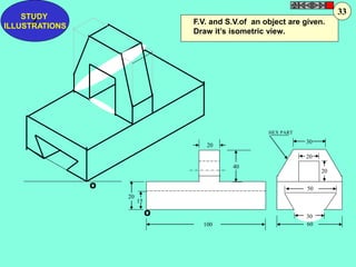
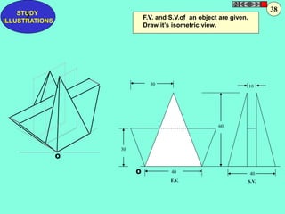
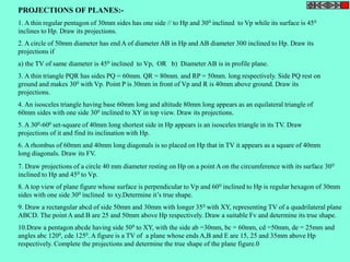
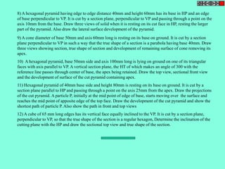
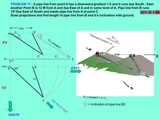
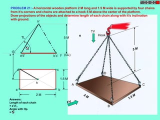
![Problem No.10: Point P is 40 mm and 30 mm from horizontal
and vertical axes respectively.Draw Hyperbola through it.
P
O
40 mm
2
2 1 1 2 3
30 mm
1
2
3
1
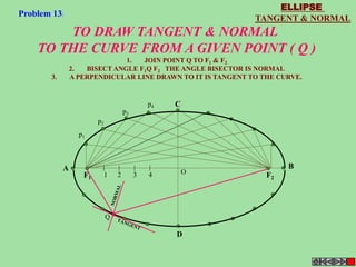
HYPERBOLA
THROUGH A POINT
OF KNOWN CO-ORDINATES
Solution Steps:
1) Extend horizontal
line from P to right side.
2) Extend vertical line
from P upward.
3) On horizontal line
from P, mark some points
taking any distance and
name them after P-1,
2,3,4 etc.
4) Join 1-2-3-4 points
to pole O. Let them cut
part [P-B] also at 1,2,3,4
points.
5) From horizontal
1,2,3,4 draw vertical
lines downwards and
6) From vertical 1,2,3,4
points [from P-B] draw
horizontal lines.
7) Line from 1
horizontal and line from
1 vertical will meet at
P1.Similarly mark P2, P3,
P4 points.
8) Repeat the procedure
by marking four points
on upward vertical line
from P and joining all
those to pole O. Name
this points P6, P7, P8 etc.
and join them by smooth
curve.](https://image.slidesharecdn.com/engineering-graphics-chetas-141018070130-conversion-gate01/85/Engineering-graphics-46-320.jpg)
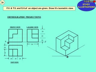
![A1
A2
A3
A B
A4
A5
A6
A7
P
p1 p2
p3
p4
p5
p6 p7
p8
1 2 3
4 5 6 7
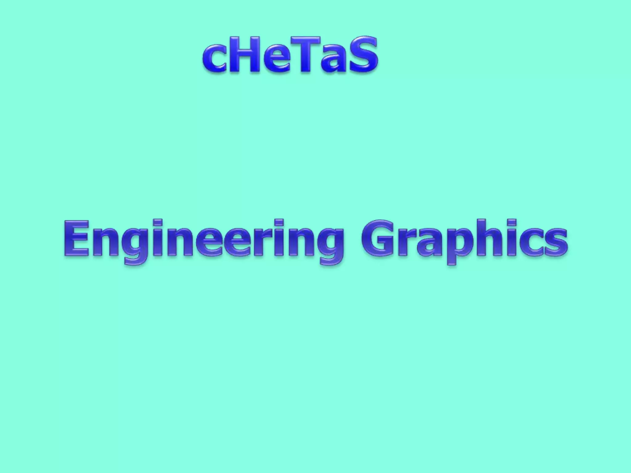
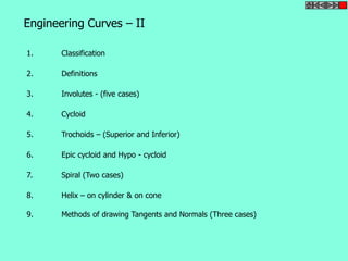
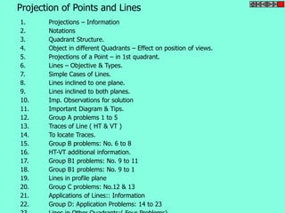
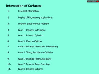
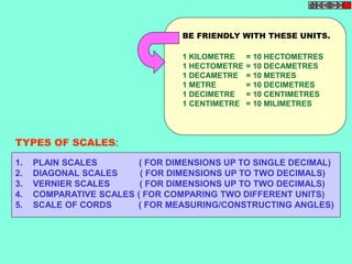
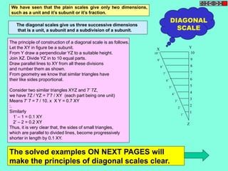
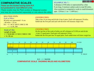
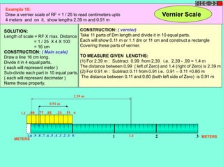
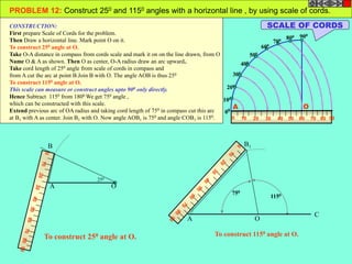
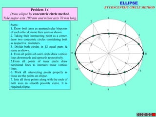
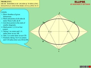
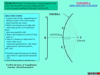
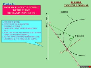
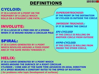
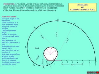
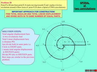
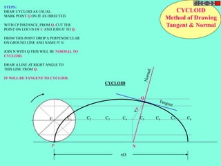
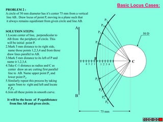
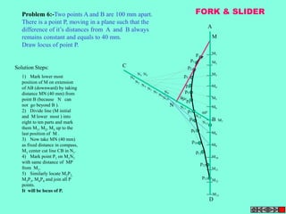
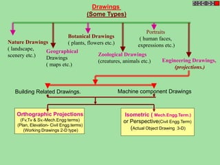
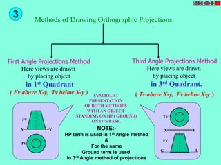
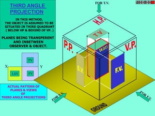
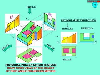
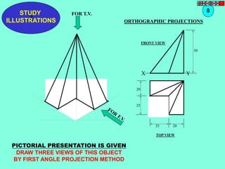
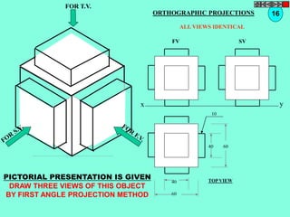
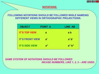
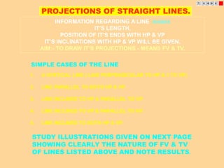
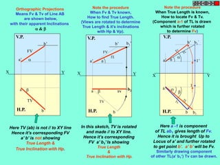
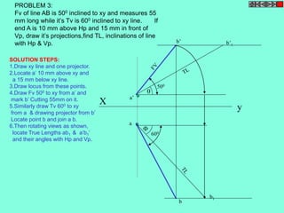
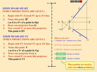
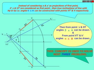
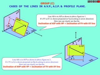
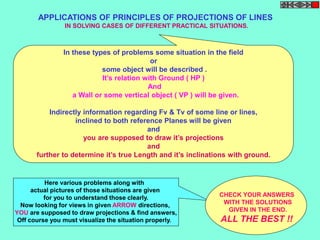
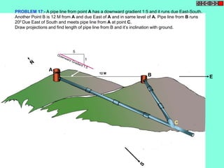
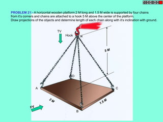
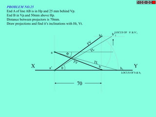
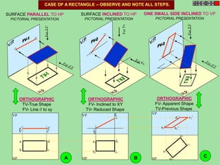
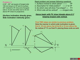
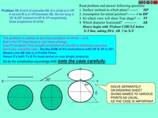
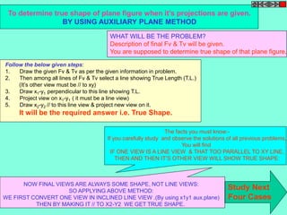
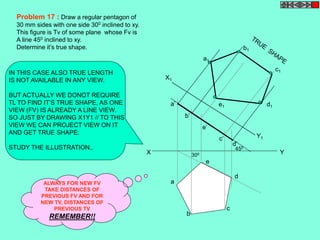
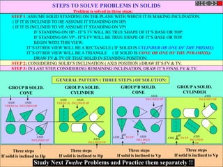
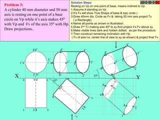
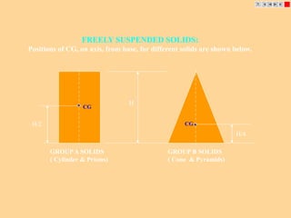
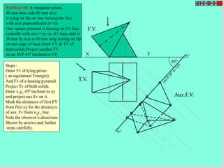
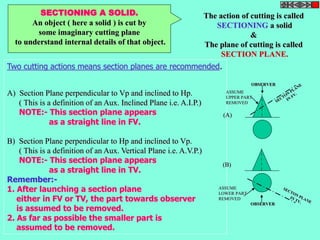
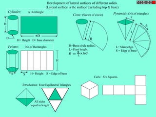
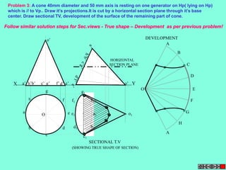
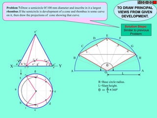
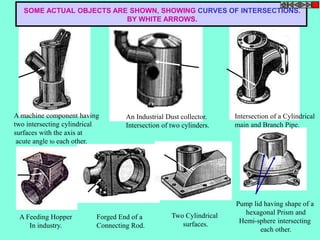
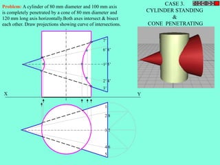
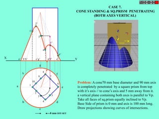
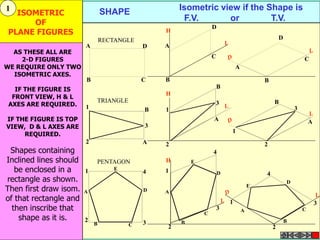
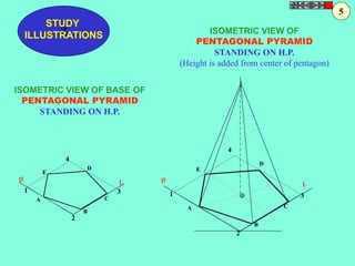
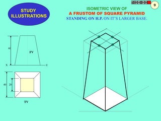
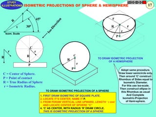
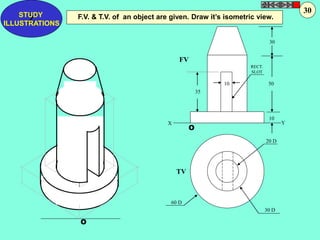
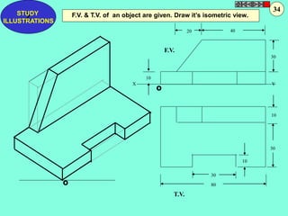
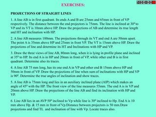
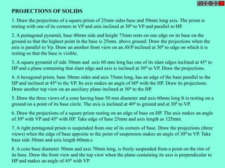
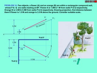
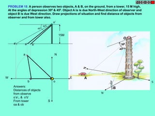
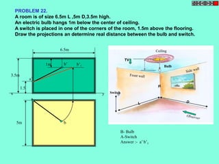
Problem 9:
Rod AB, 100 mm long, revolves in clockwise direction for one revolution.
Meanwhile point P, initially on A starts moving towards B and reaches B.
Draw locus of point P.
ROTATING LINK
1) AB Rod revolves around
center O for one revolution and
point P slides along AB rod and
reaches end B in one
revolution.
2) Divide circle in 8 number of
equal parts and name in arrow
direction after A-A1, A2, A3, up
to A8.
3) Distance traveled by point P
is AB mm. Divide this also into 8
number of equal parts.
4) Initially P is on end A. When
A moves to A1, point P goes
one linear division (part) away
from A1. Mark it from A1 and
name the point P1.
5) When A moves to A2, P will
be two parts away from A2
(Name it P2 ). Mark it as above
from A2.
6) From A3 mark P3 three
parts away from P3.
7) Similarly locate P4, P5, P6,
P7 and P8 which will be eight
parts away from A8. [Means P
has reached B].
8) Join all P points by smooth
curve. It will be locus of P](https://image.slidesharecdn.com/engineering-graphics-chetas-141018070130-conversion-gate01/85/Engineering-graphics-81-320.jpg)
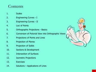
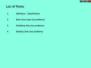
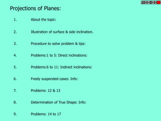
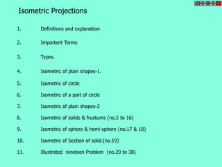
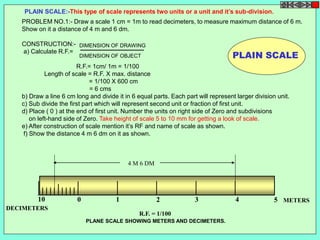
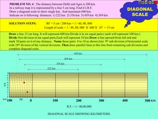
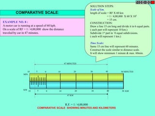
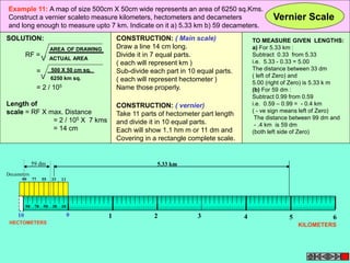
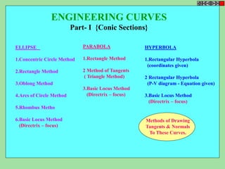
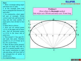
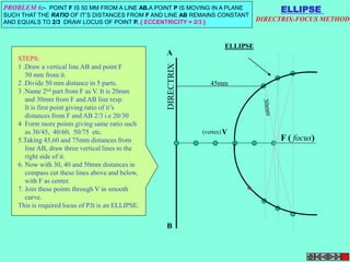
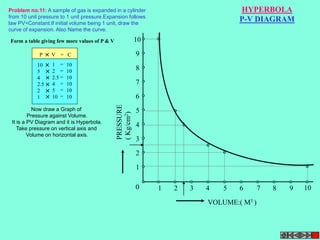
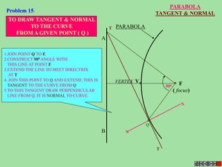
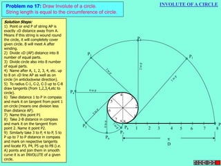
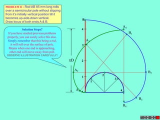
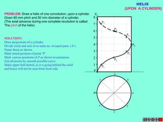
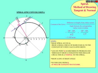
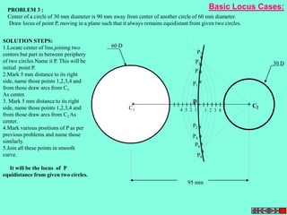
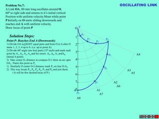
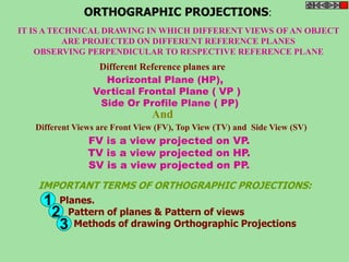
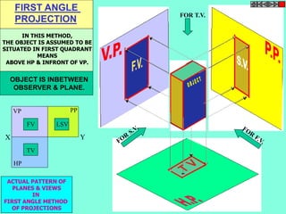
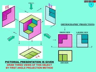
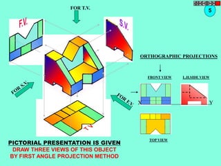
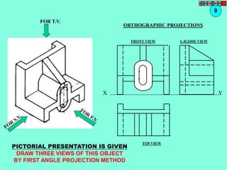
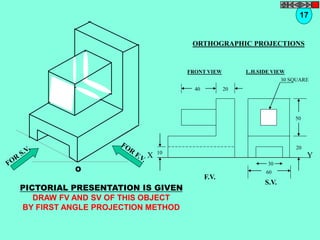
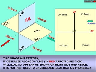
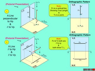
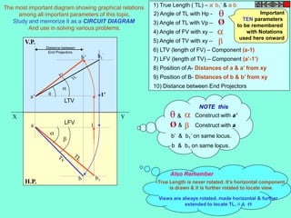
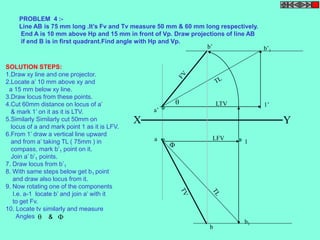
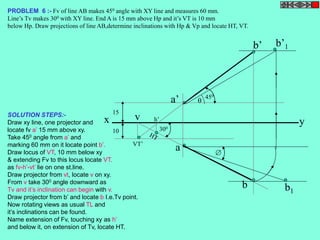
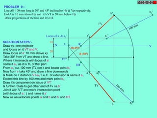
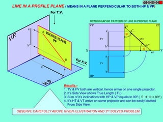
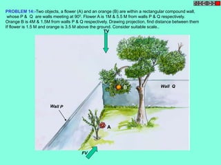
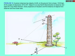
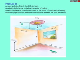
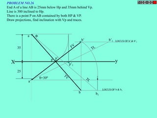
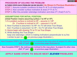
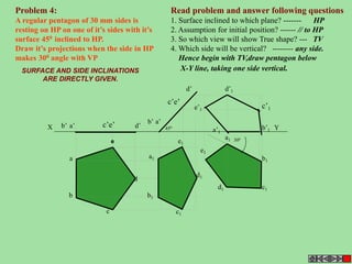
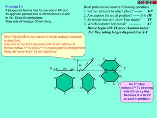
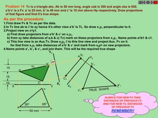
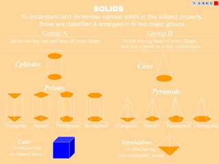
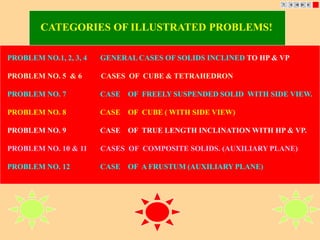
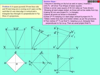
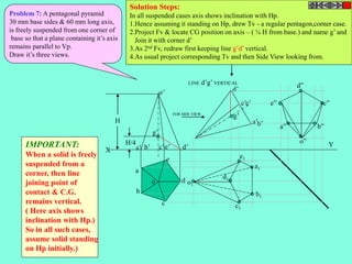
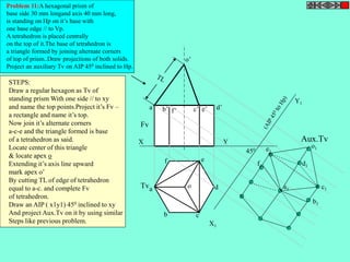
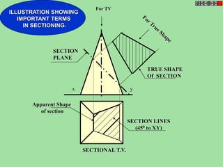
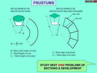
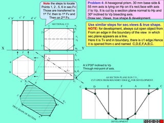
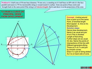
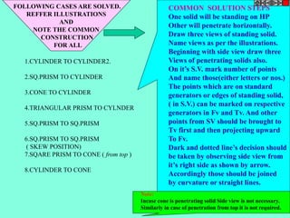
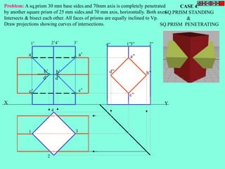
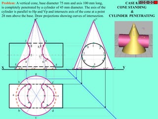
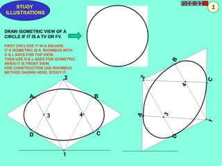
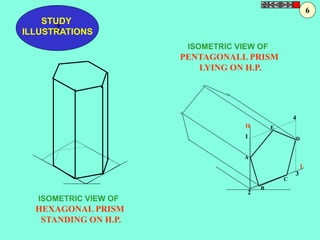
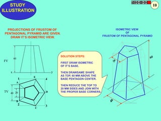
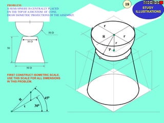
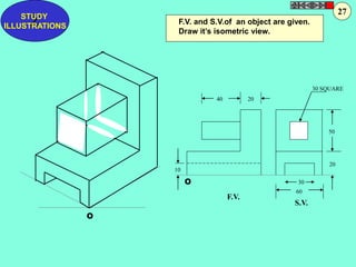
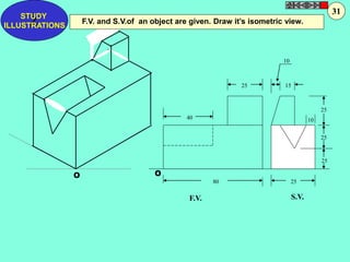
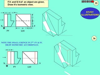
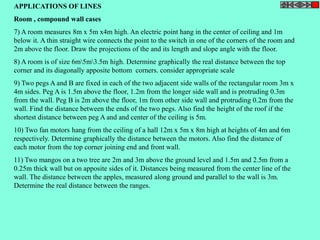
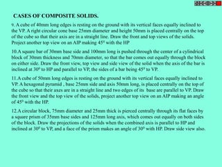
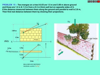
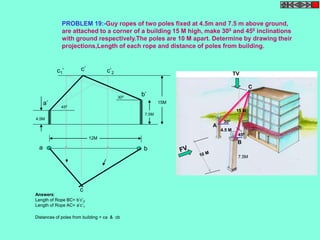
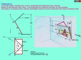
![Problem 10 :
Rod AB, 100 mm long, revolves in clockwise direction for one revolution.
Meanwhile point P, initially on A starts moving towards B, reaches B
And returns to A in one revolution of rod.
Draw locus of point P.
Solution Steps
A1
A2
ROTATING LINK
A3
A B
A4
+ + + +
A5
A6
A7
P
p1
p2
p3
p4
p5
p6
p7
p8
1 7 2 6 3 5 4
1) AB Rod revolves around center O
for one revolution and point P slides
along rod AB reaches end B and
returns to A.
2) Divide circle in 8 number of equal
parts and name in arrow direction
after A-A1, A2, A3, up to A8.
3) Distance traveled by point P is AB
plus AB mm. Divide AB in 4 parts so
those will be 8 equal parts on return.
4) Initially P is on end A. When A
moves to A1, point P goes one
linear division (part) away from A1.
Mark it from A1 and name the point
P1.
5) When A moves to A2, P will be
two parts away from A2 (Name it P2
). Mark it as above from A2.
6) From A3 mark P3 three parts
away from P3.
7) Similarly locate P4, P5, P6, P7
and P8 which will be eight parts away
from A8. [Means P has reached B].
8) Join all P points by smooth curve.
It will be locus of P
The Locus will follow the loop
path two times in one revolution.](https://image.slidesharecdn.com/engineering-graphics-chetas-141018070130-conversion-gate01/85/Engineering-graphics-82-320.jpg)
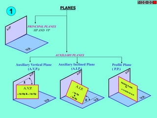
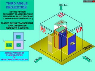

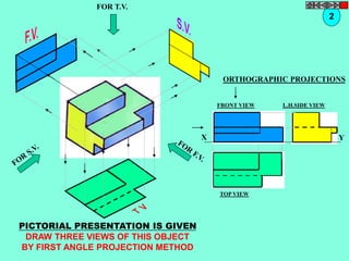
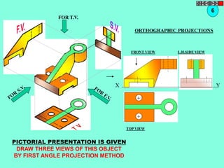
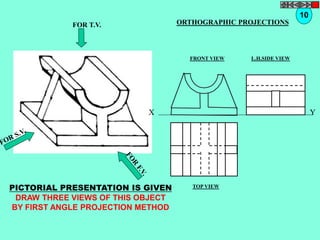
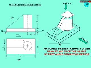
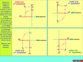
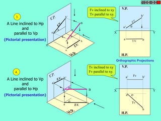
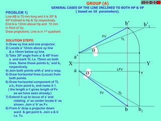
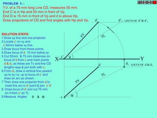
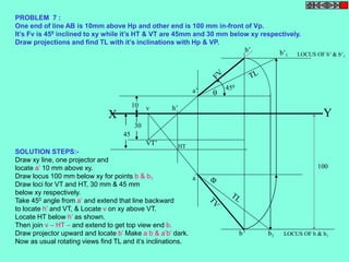
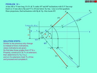
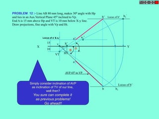
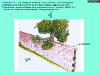
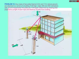
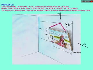
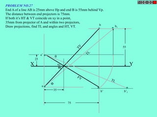
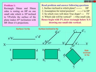
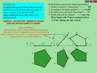
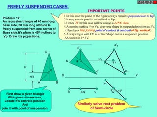
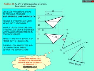
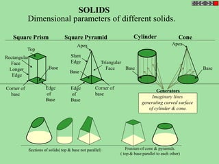
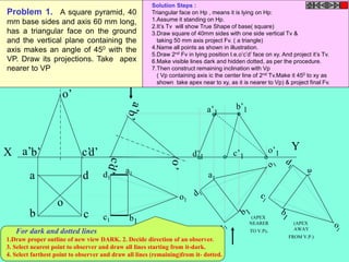
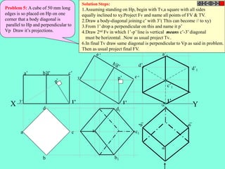
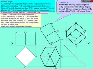
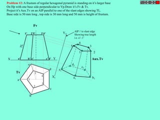
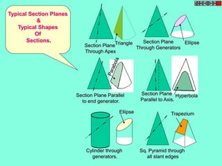
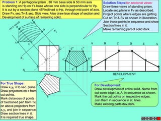
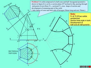
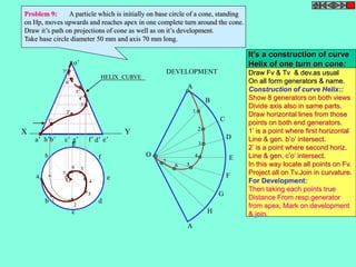
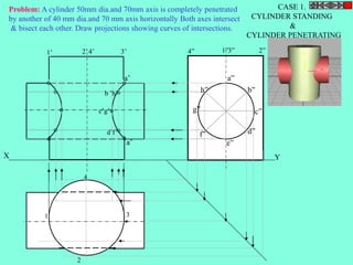
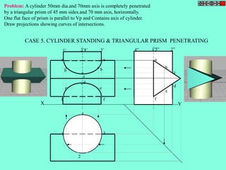
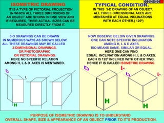
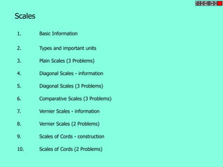
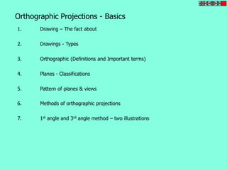
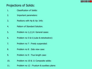
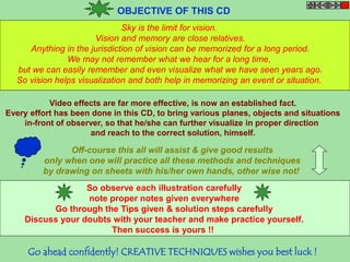
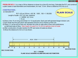
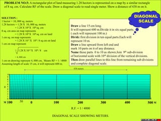
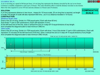
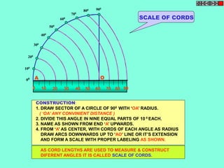
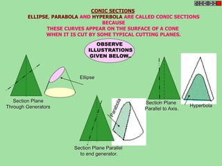
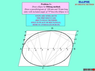
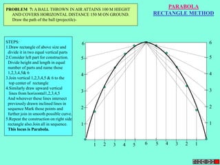
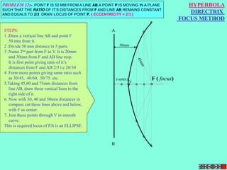
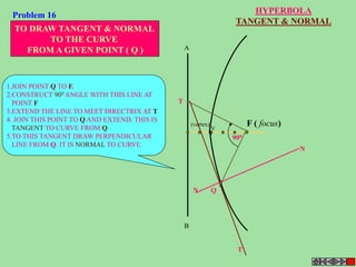
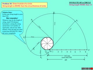
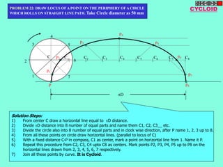
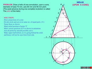
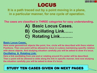
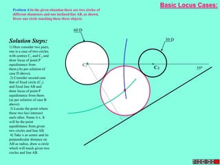
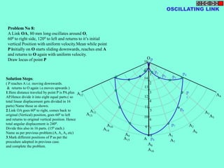
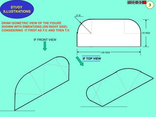
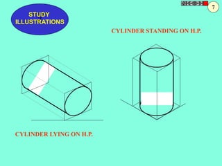
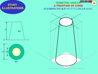
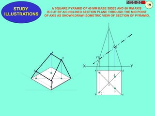
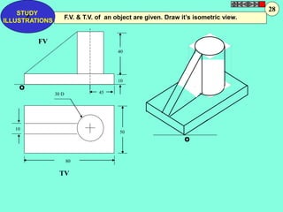
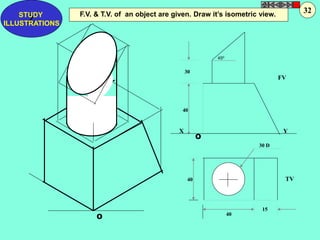
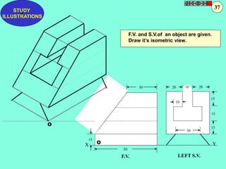
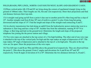
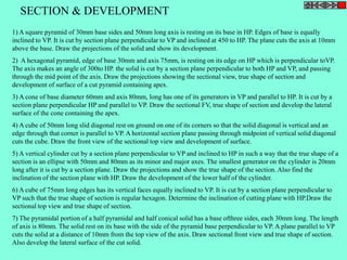
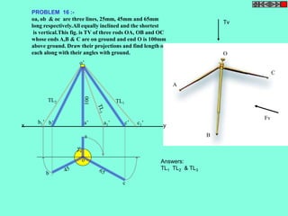
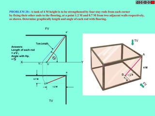
![ISOMETRIC VIEW ISOMETRIC PROJECTION
H
H
TYPES OF ISOMETRIC DRAWINGS
Drawn by using Isometric scale
( Reduced dimensions )
Drawn by using True scale
( True dimensions )
450
300
0
1
2
3
4
0
1
2
3
D
4
A B
Isometric scale [ Line AC ]
required for Isometric Projection
C
CONSTRUCTION OF ISOM.SCALE.
From point A, with line AB draw 300 and
450 inclined lines AC & AD resp on AD.
Mark divisions of true length and from
each division-point draw vertical lines
upto AC line.
The divisions thus obtained on AC
give lengths on isometric scale.](https://image.slidesharecdn.com/engineering-graphics-chetas-141018070130-conversion-gate01/85/Engineering-graphics-229-320.jpg)
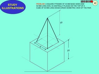
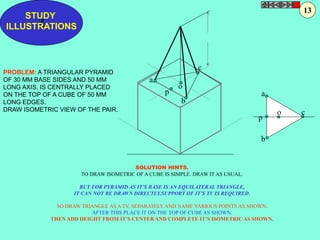
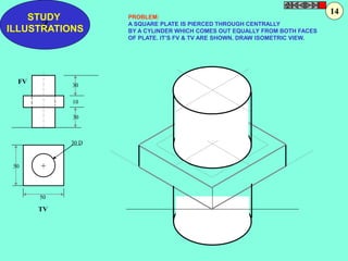
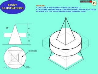

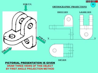
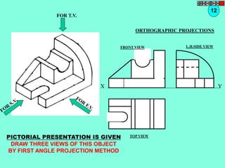
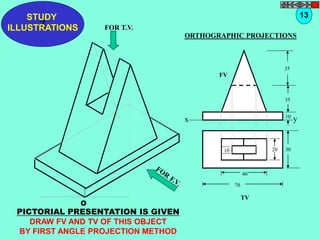
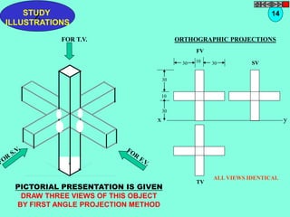
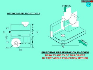
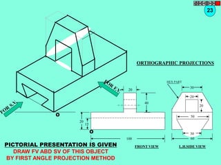
This document contains a table of contents for an engineering drawing course covering topics such as scales, engineering curves, orthographic projections, sections and developments, intersections of surfaces, and isometric projections. It includes definitions, methods, examples and practice problems for each topic. The objective stated is to use video effects to help visualize concepts in 3D and correctly solve problems through practice of drawing by hand with guidance from illustrations and notes provided throughout.


![Engineering] Drawing Curve1](https://cdn.slidesharecdn.com/ss_thumbnails/curve1-140530123909-phpapp01-thumbnail.jpg?width=640&height=640&fit=bounds)