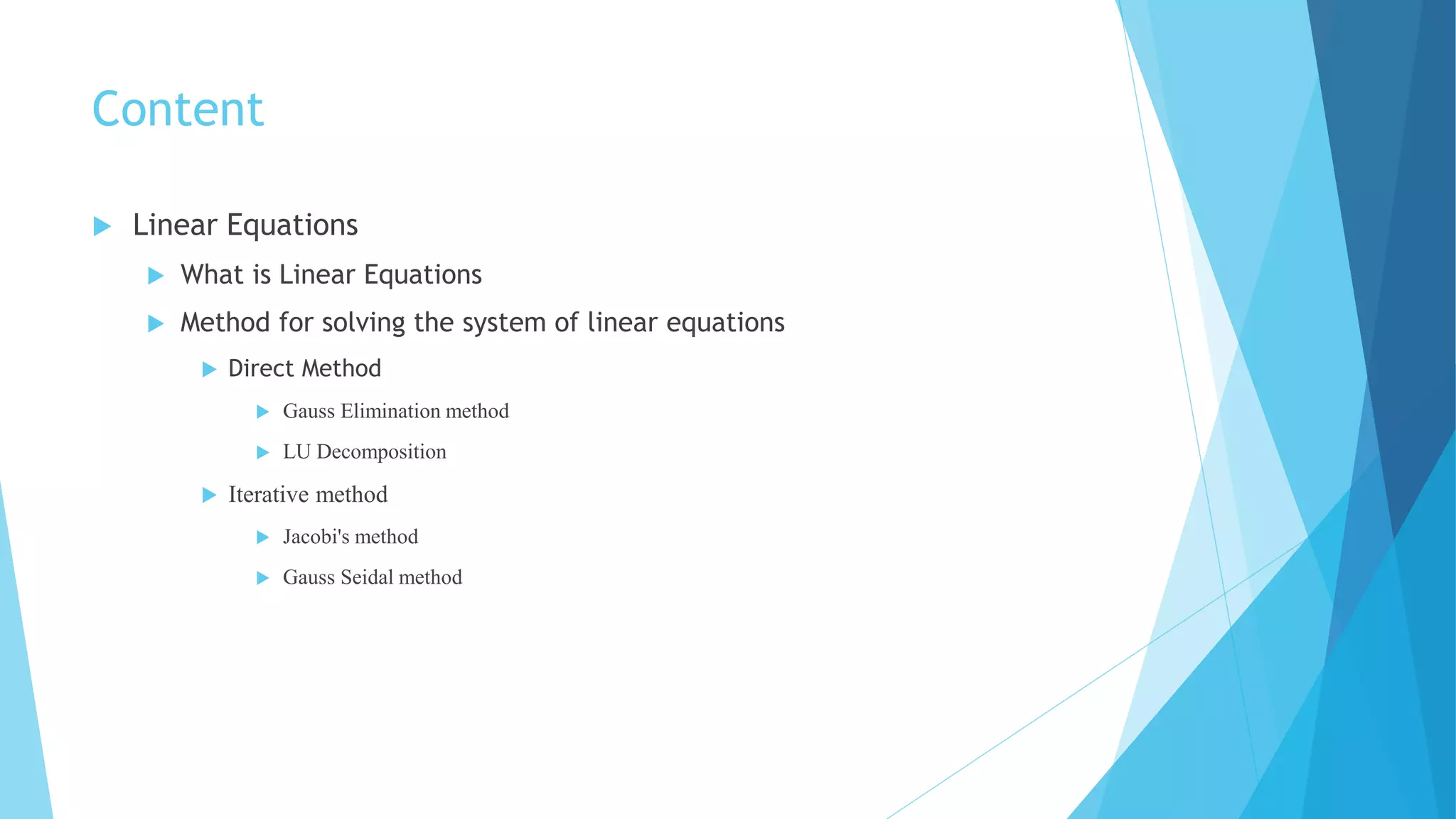
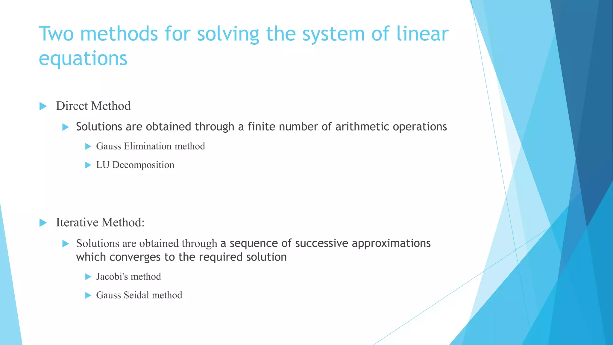
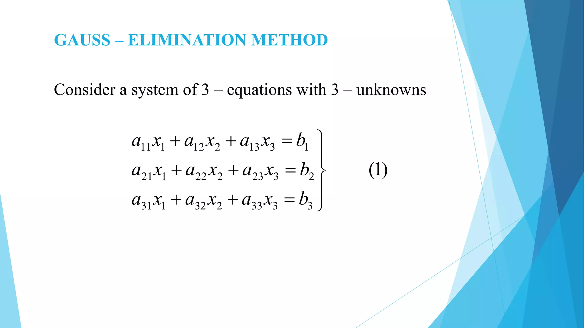
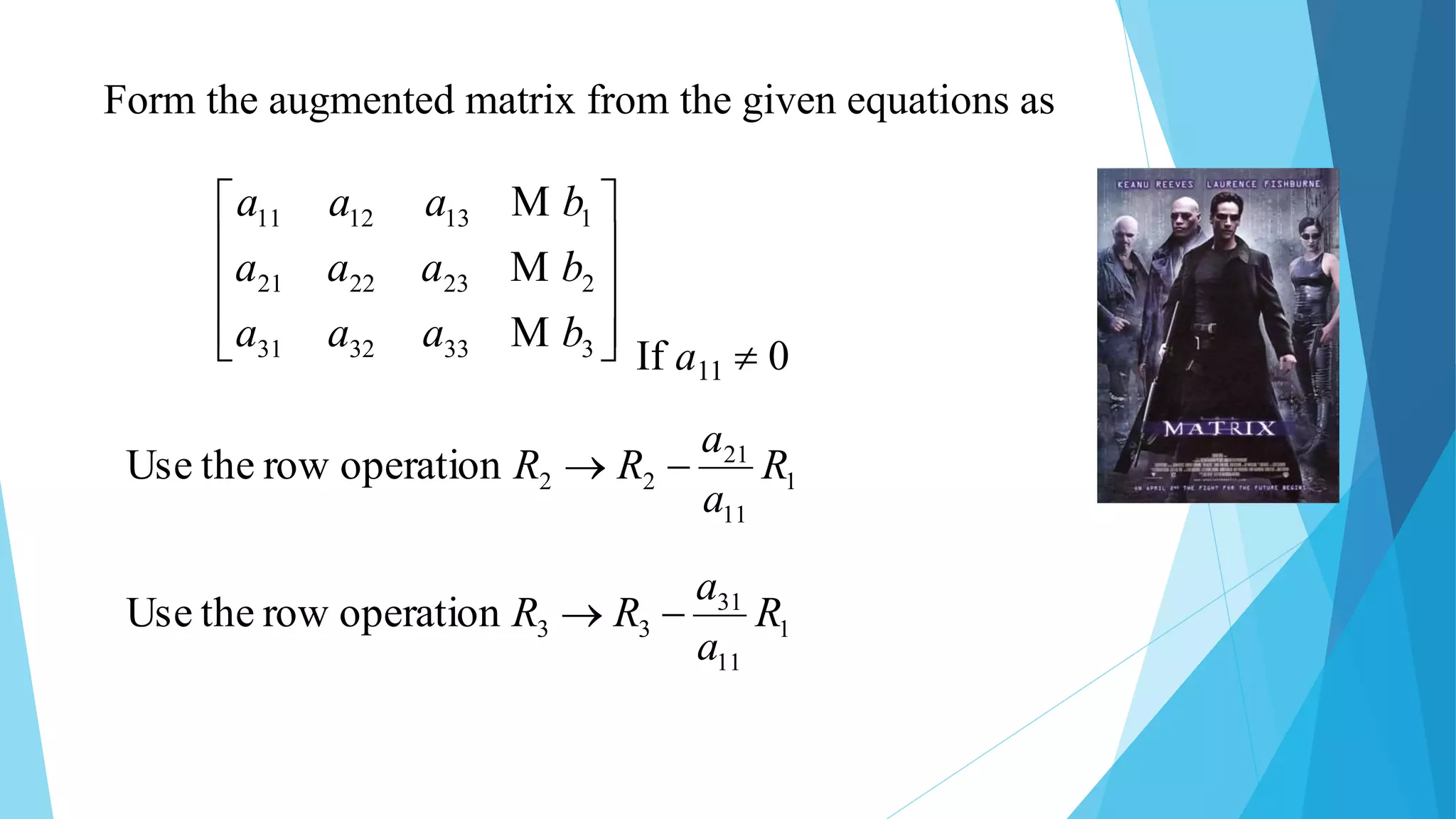
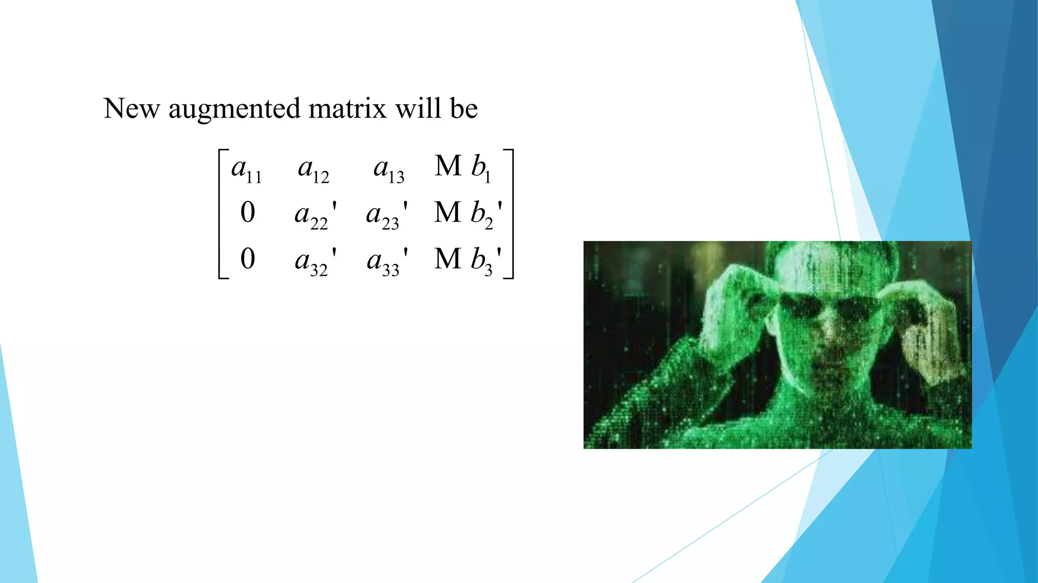
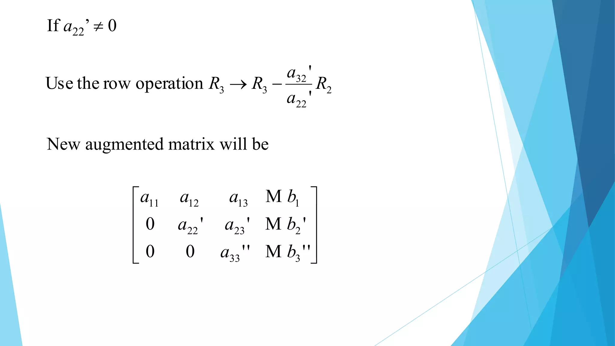
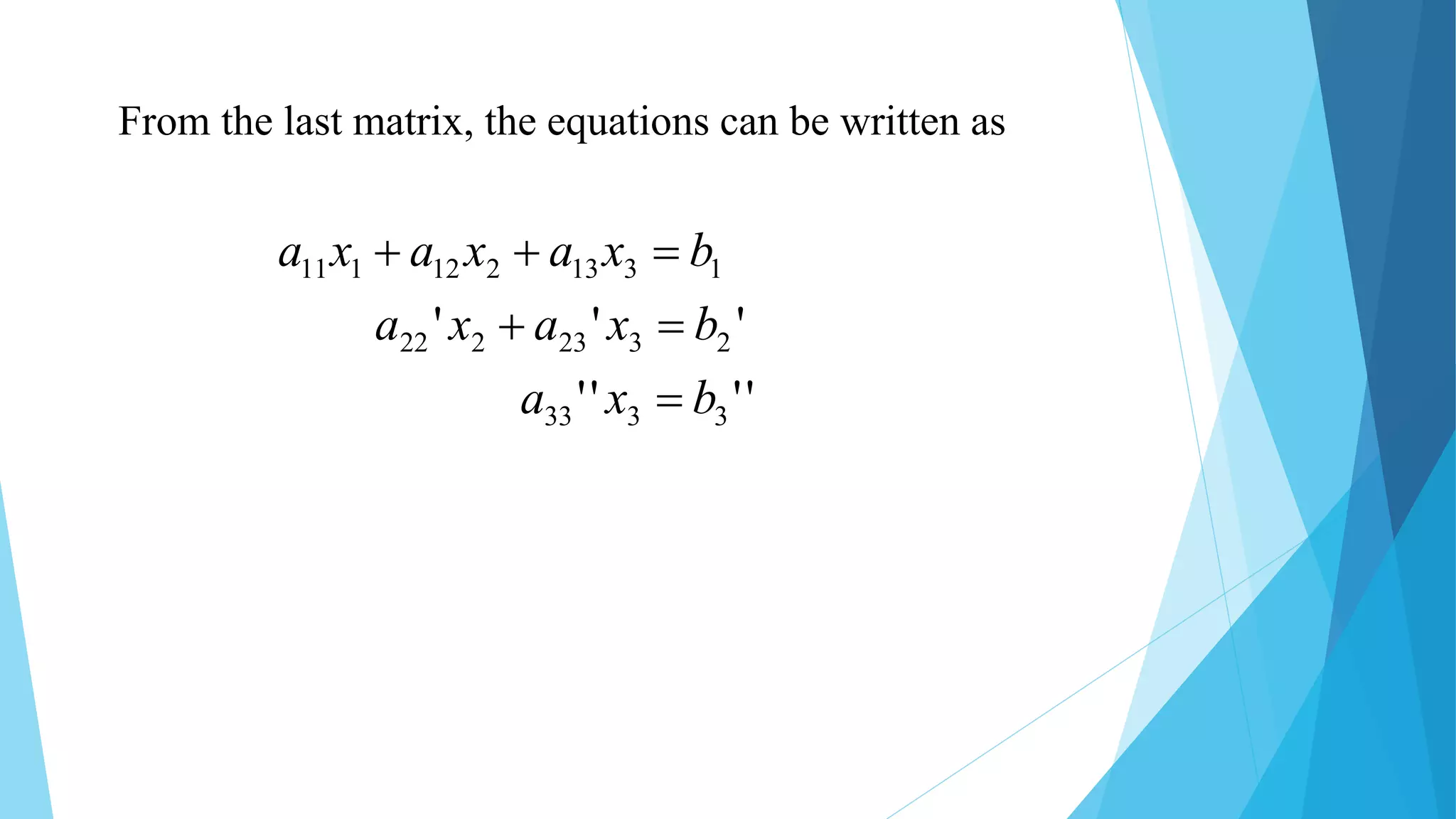
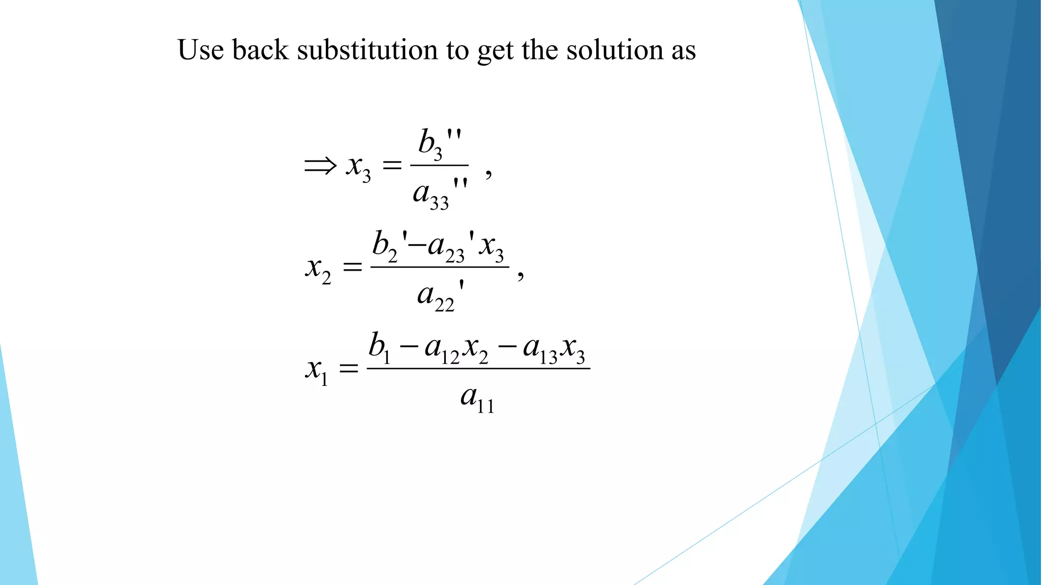
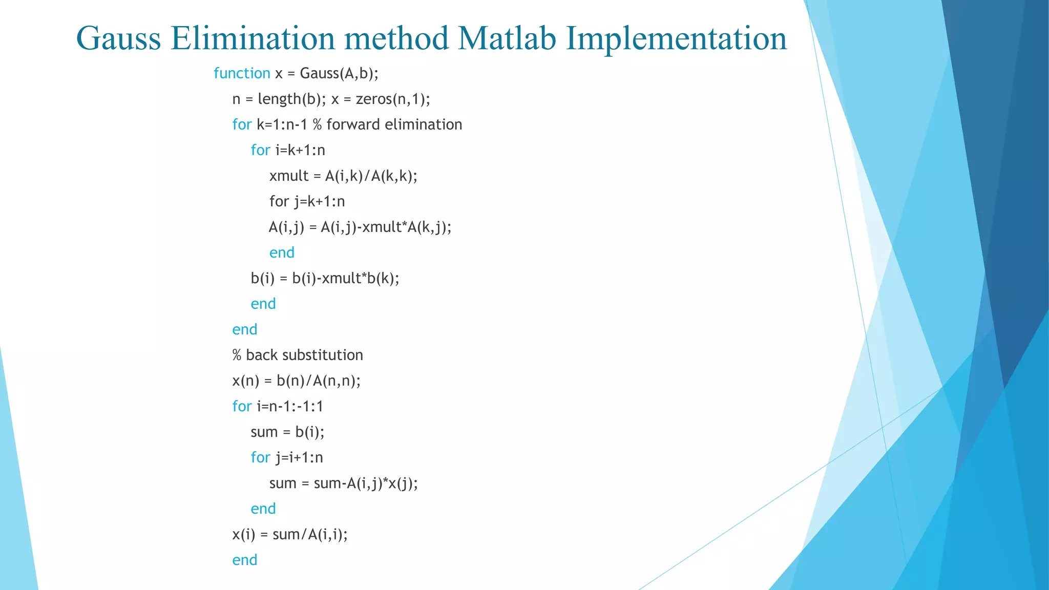
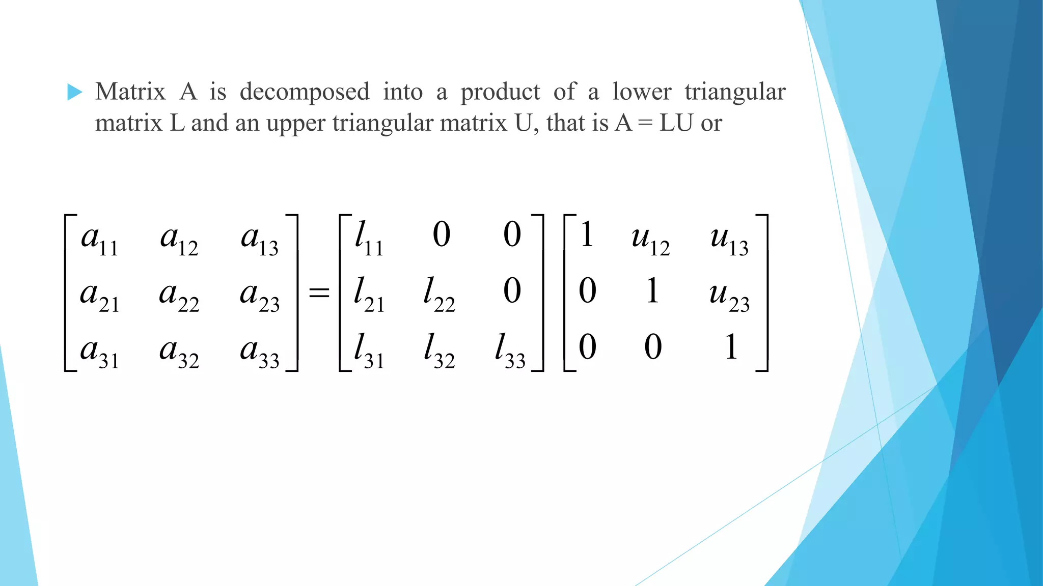
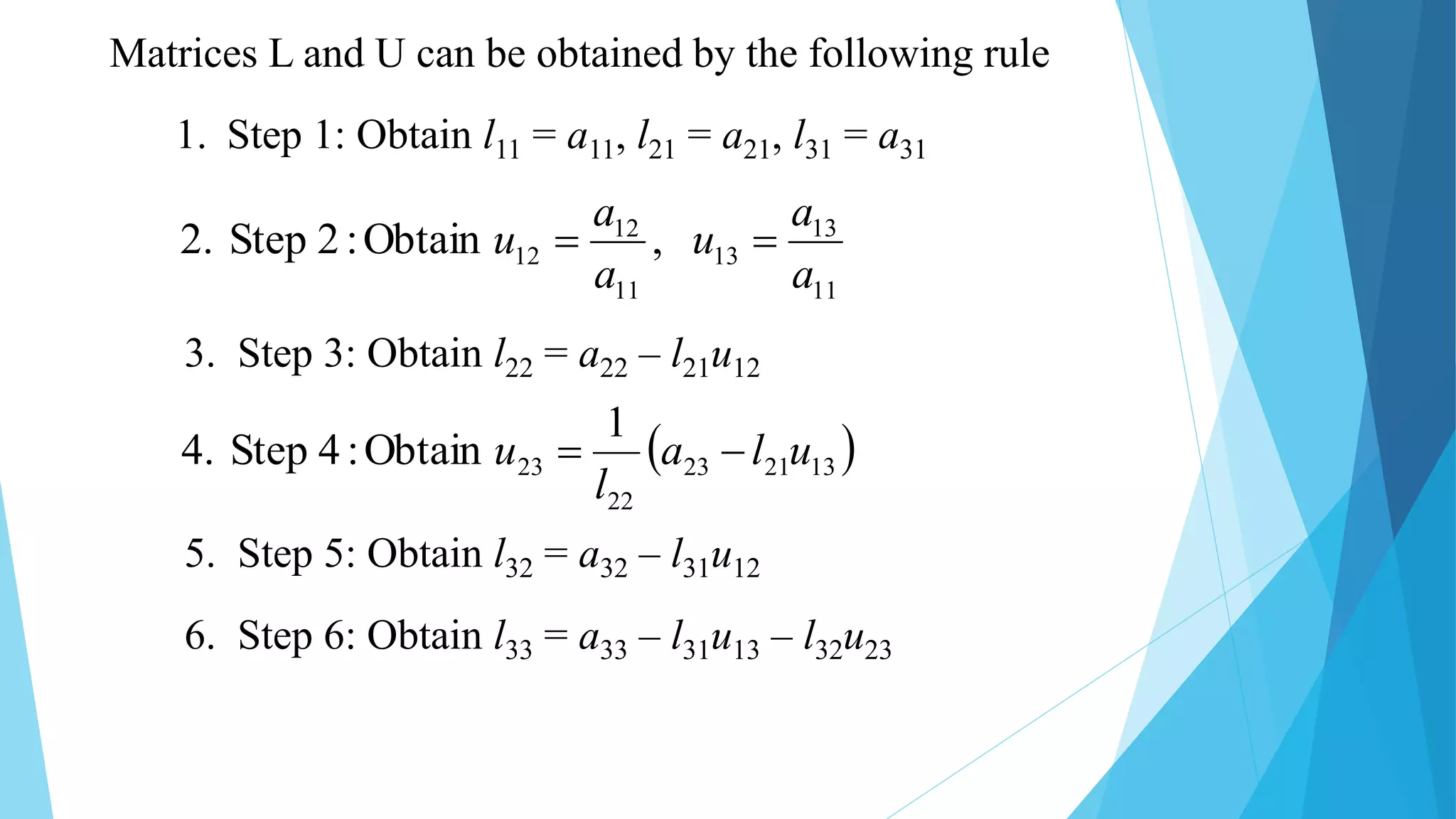
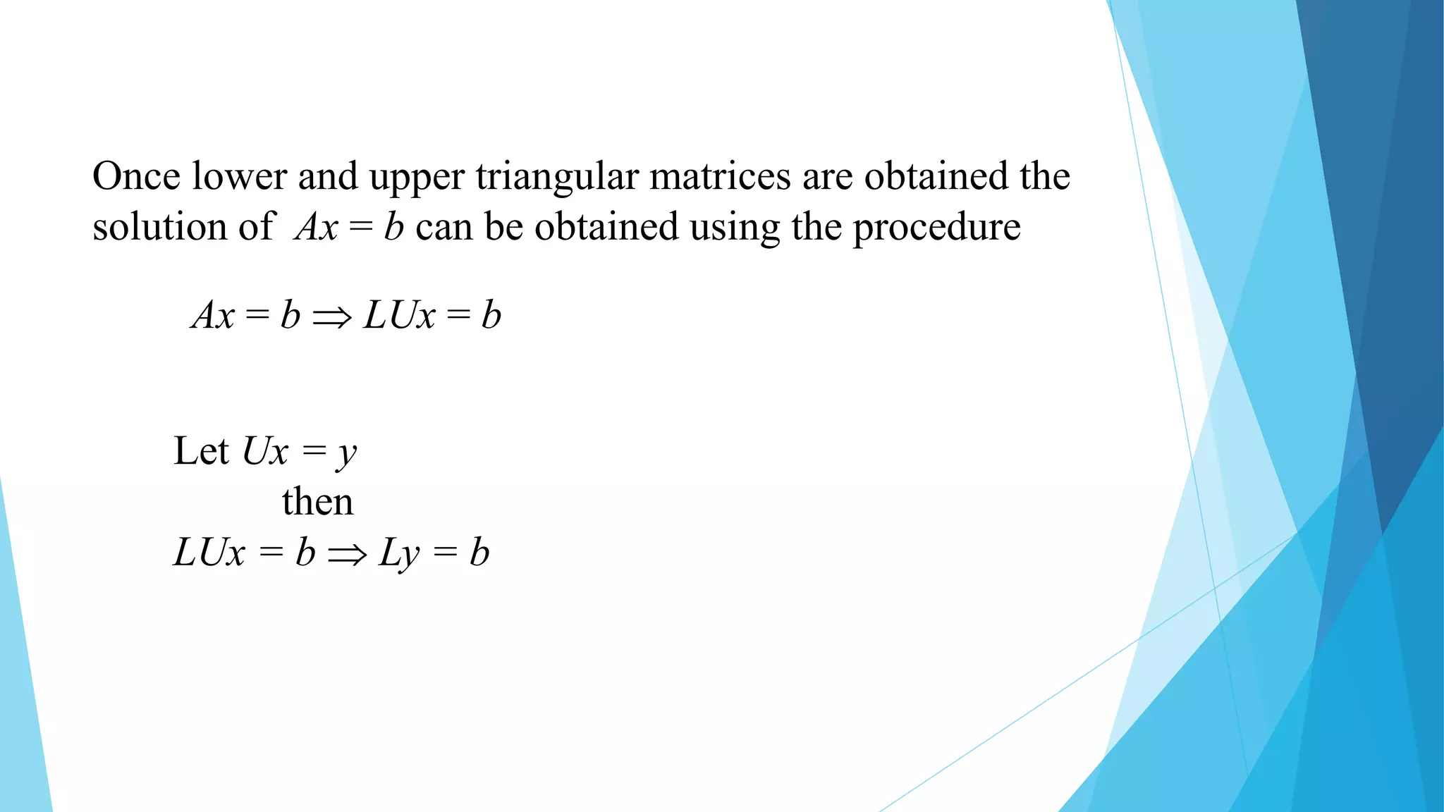
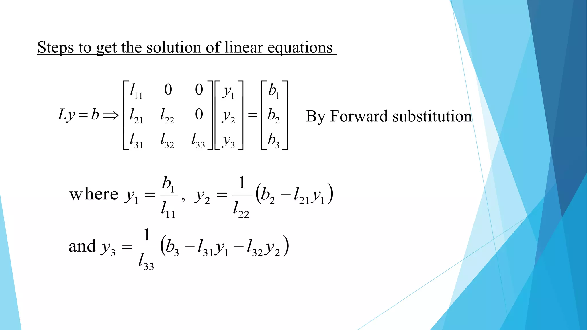
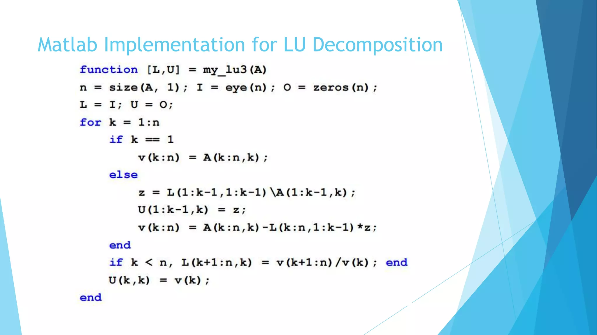
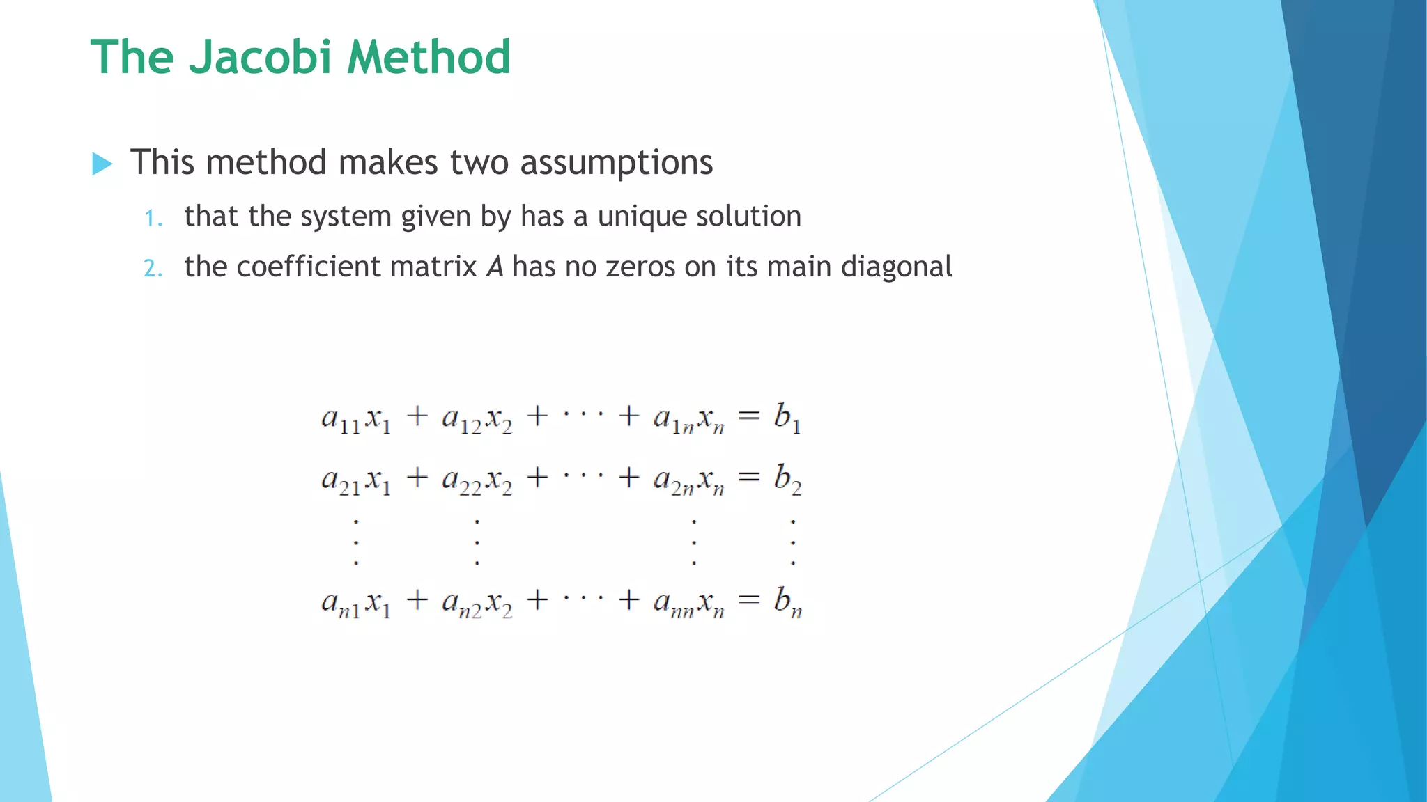
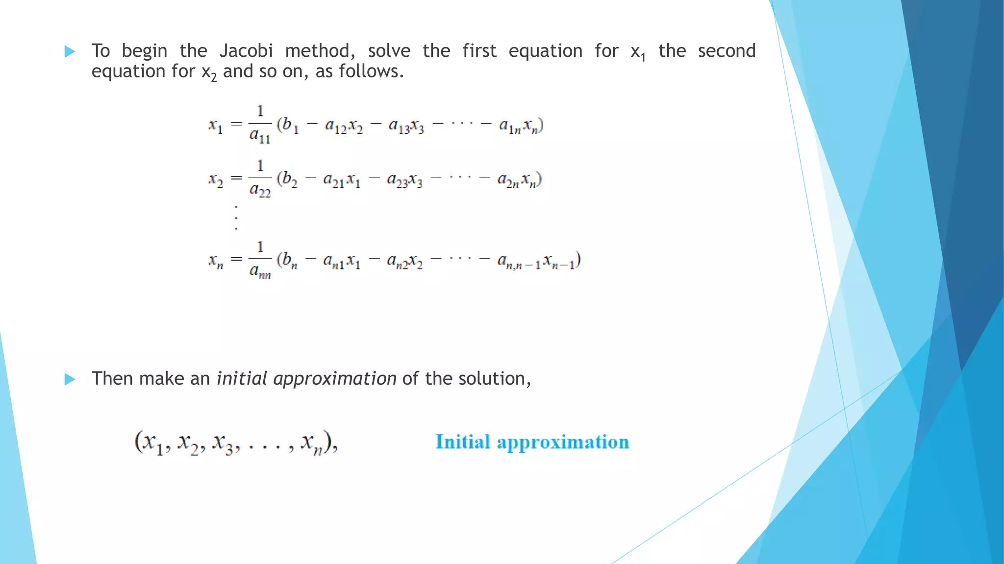
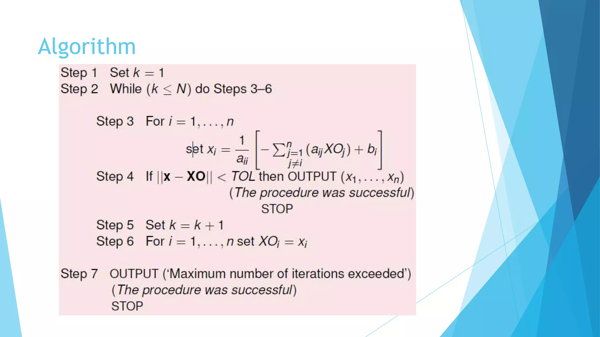
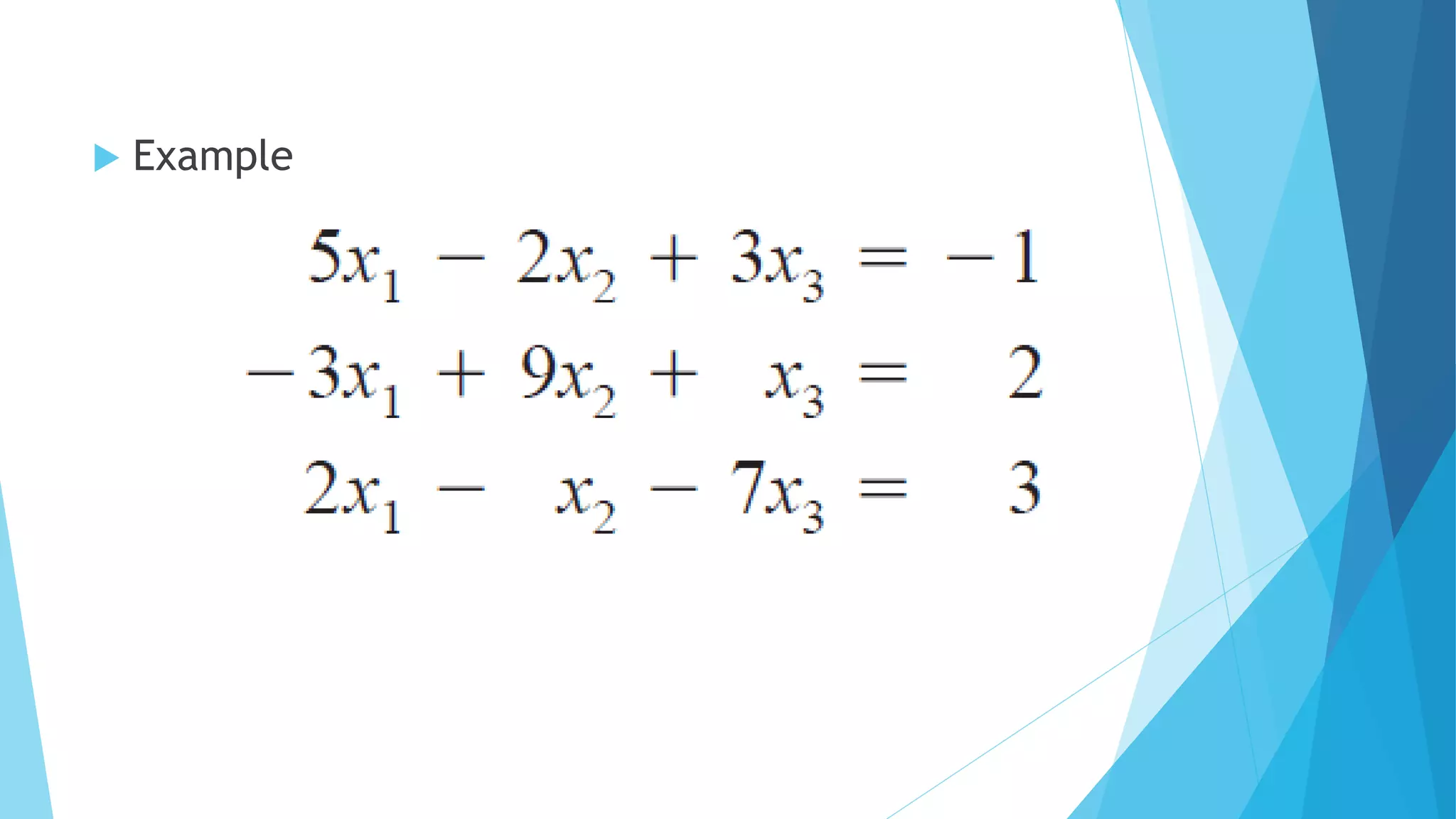
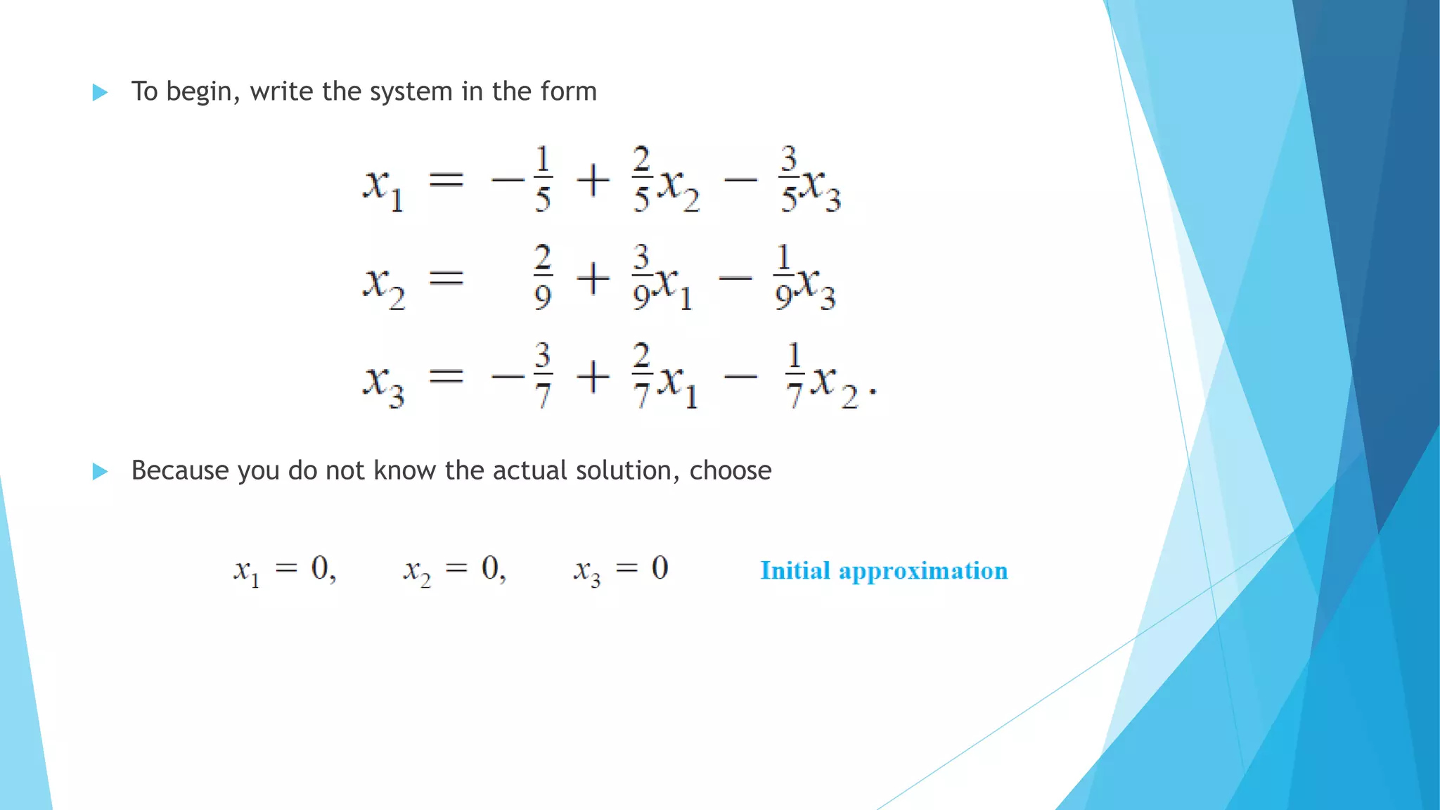
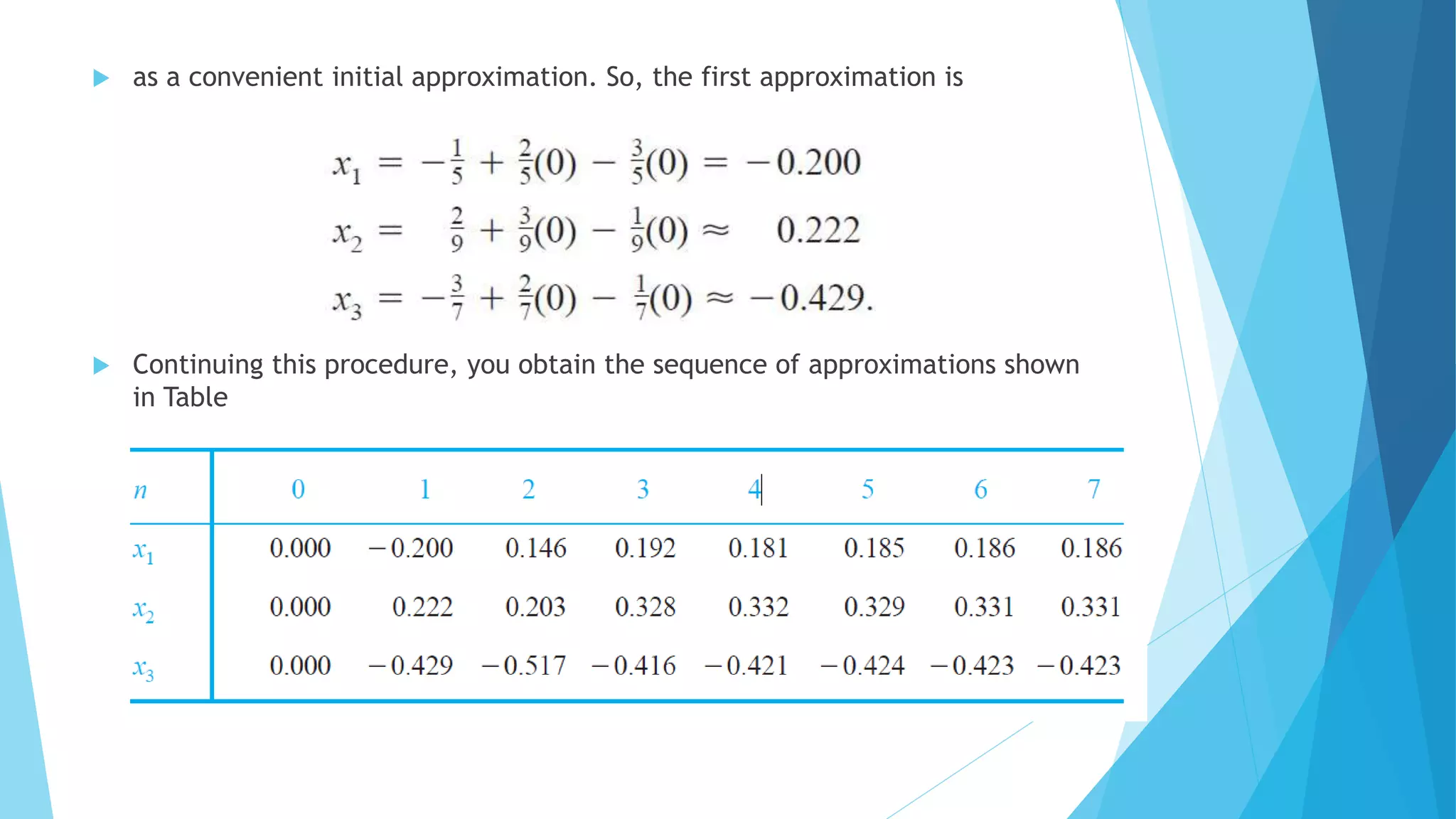
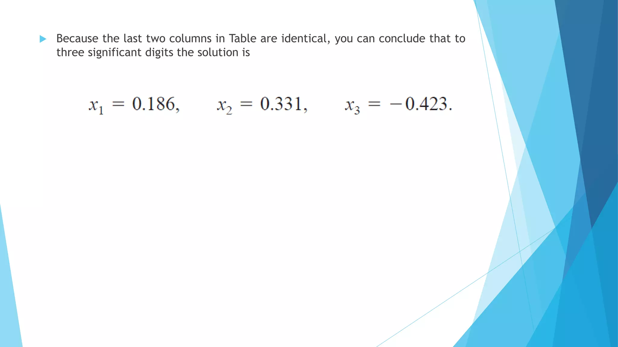
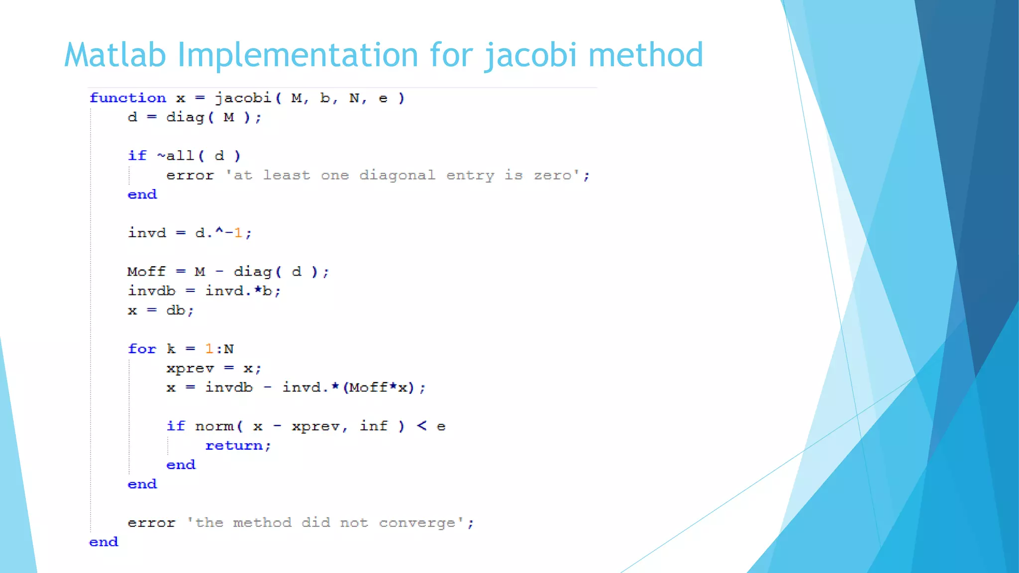
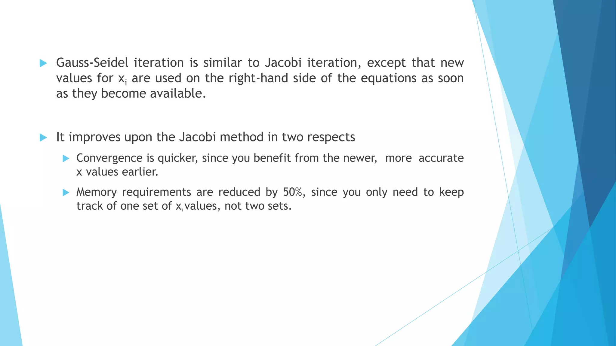
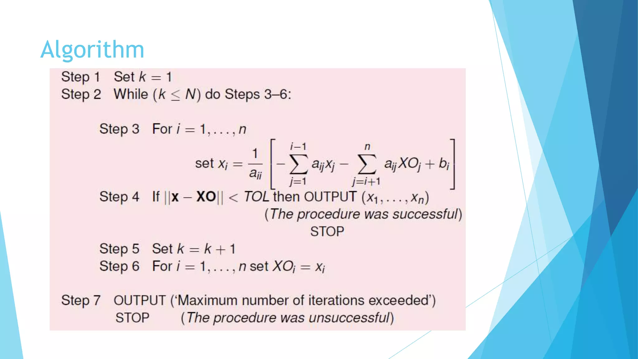
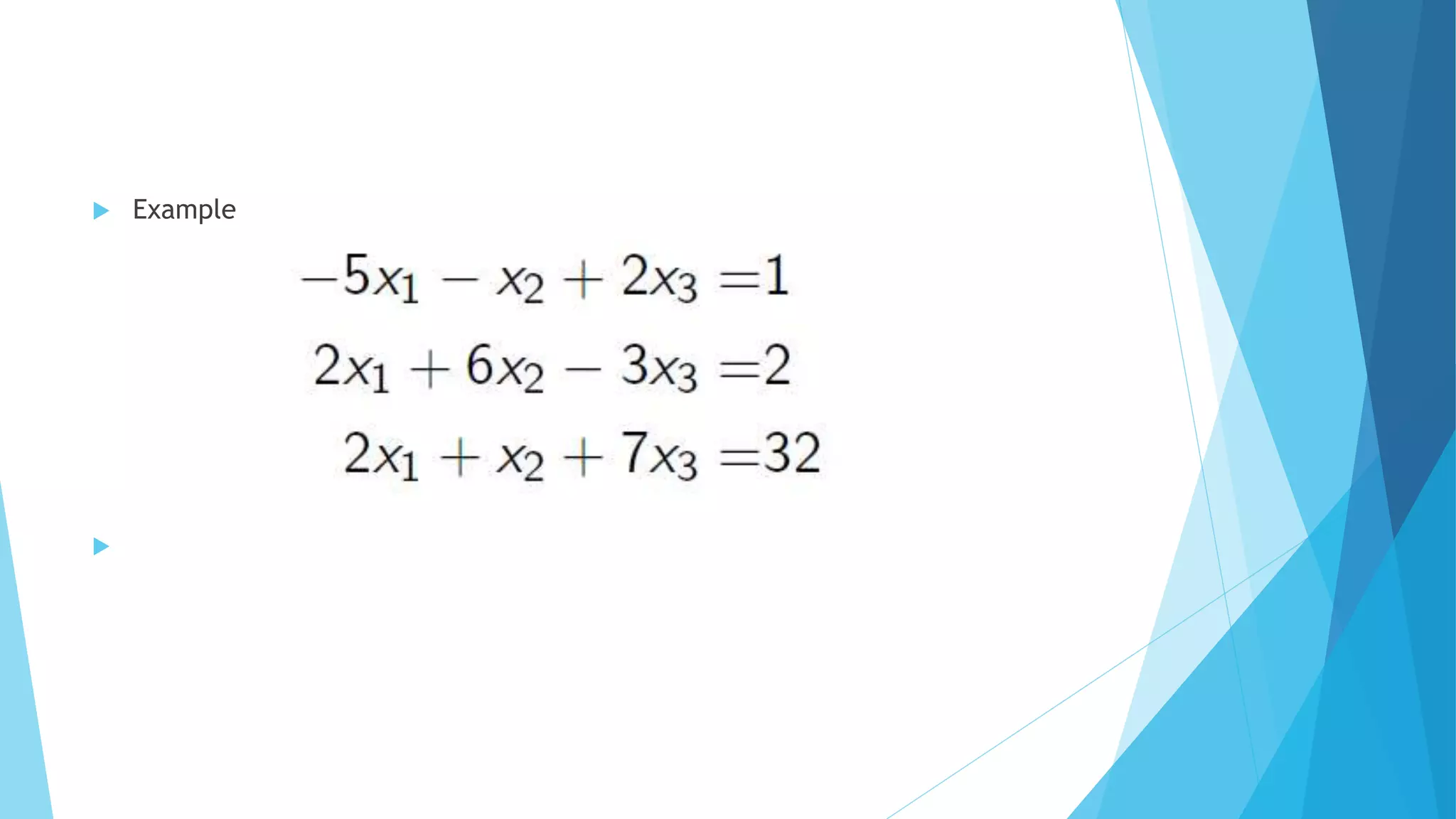
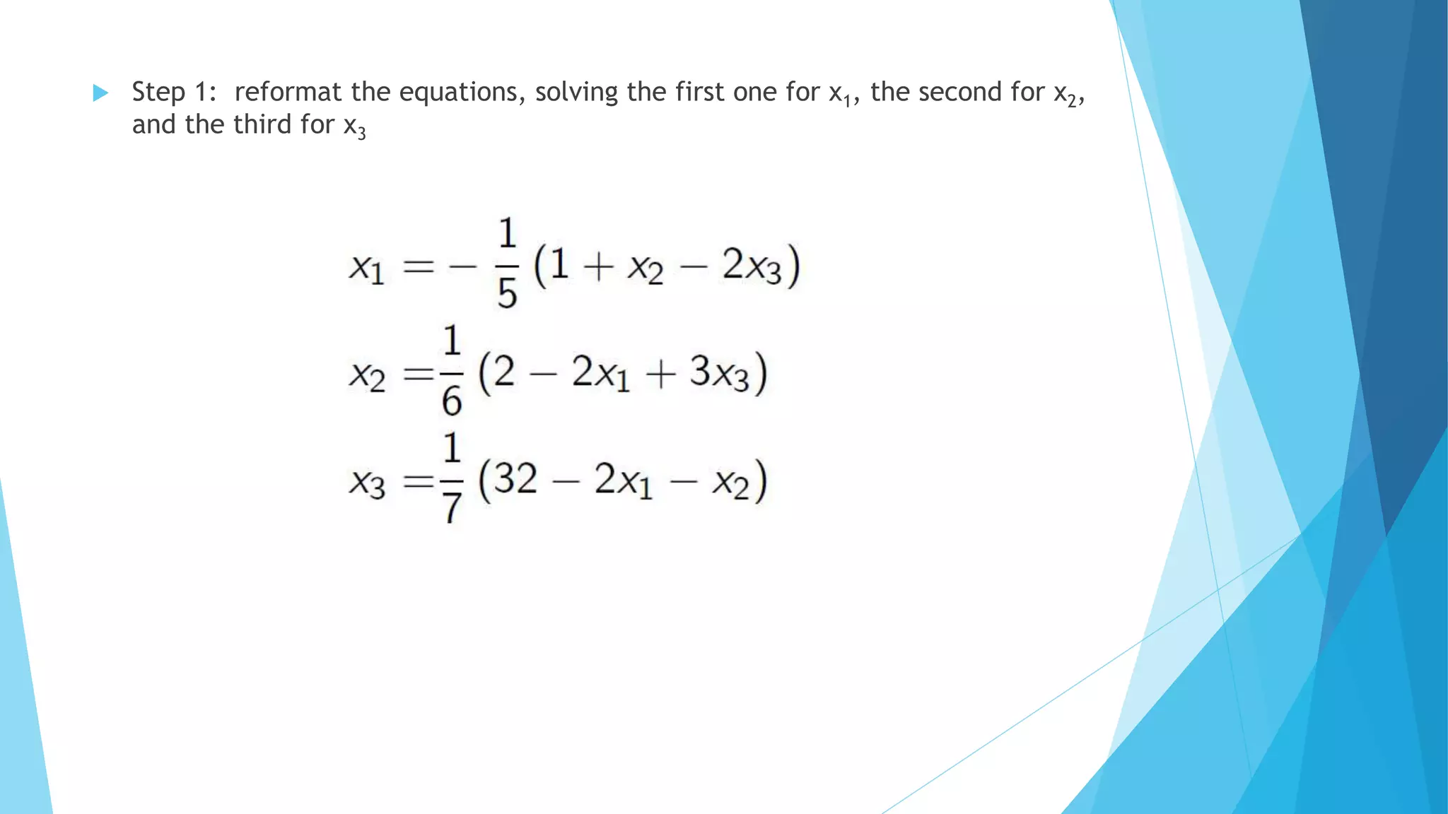
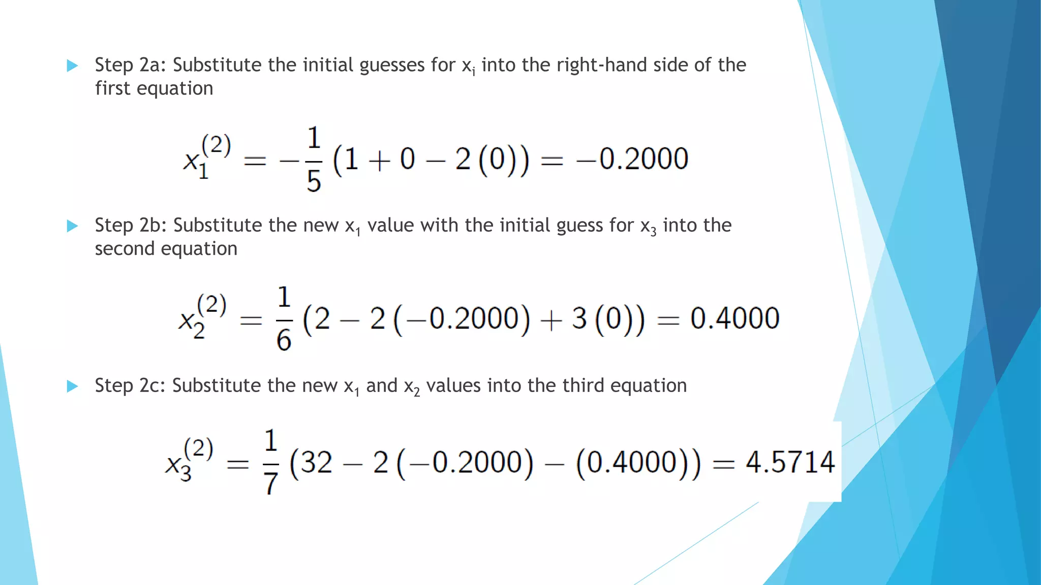
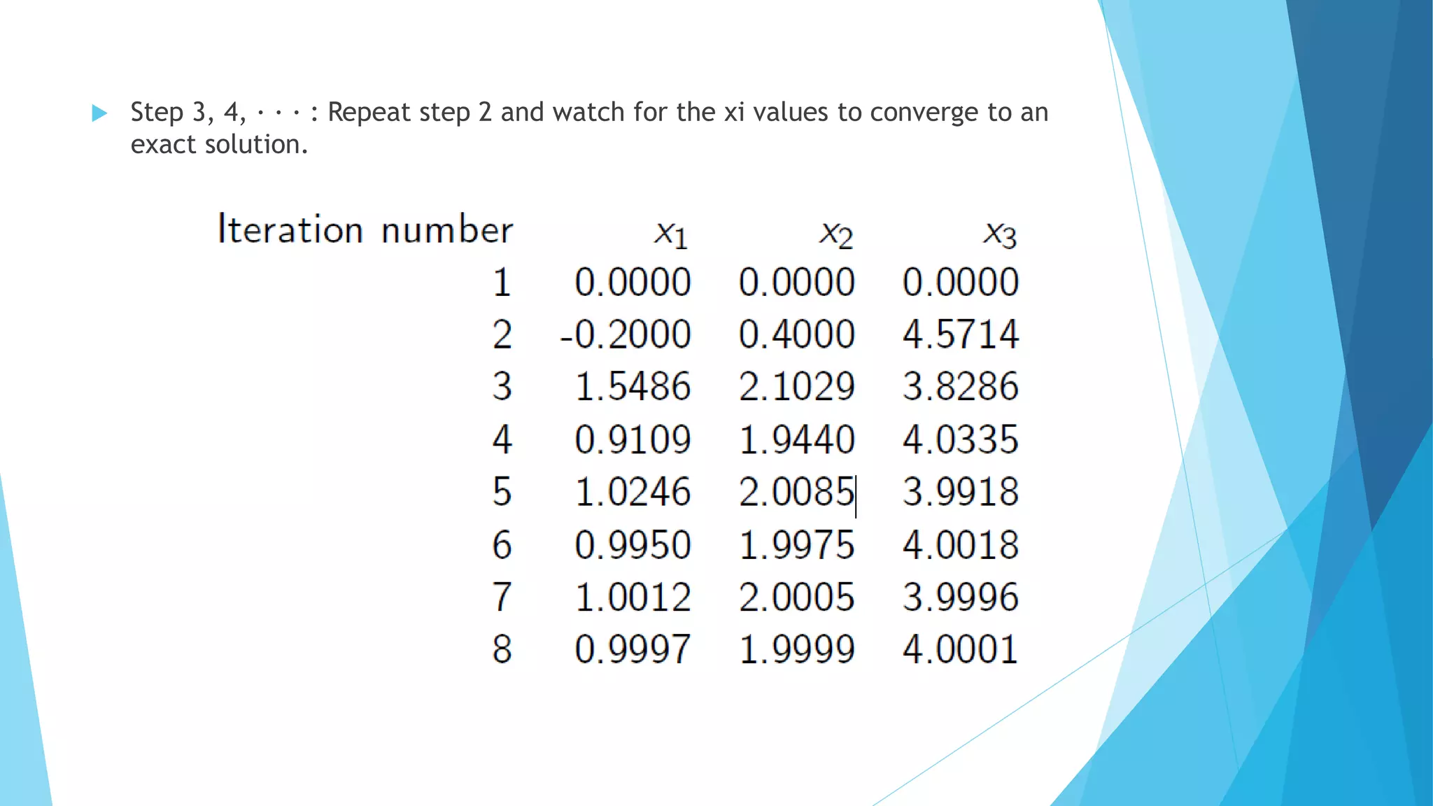
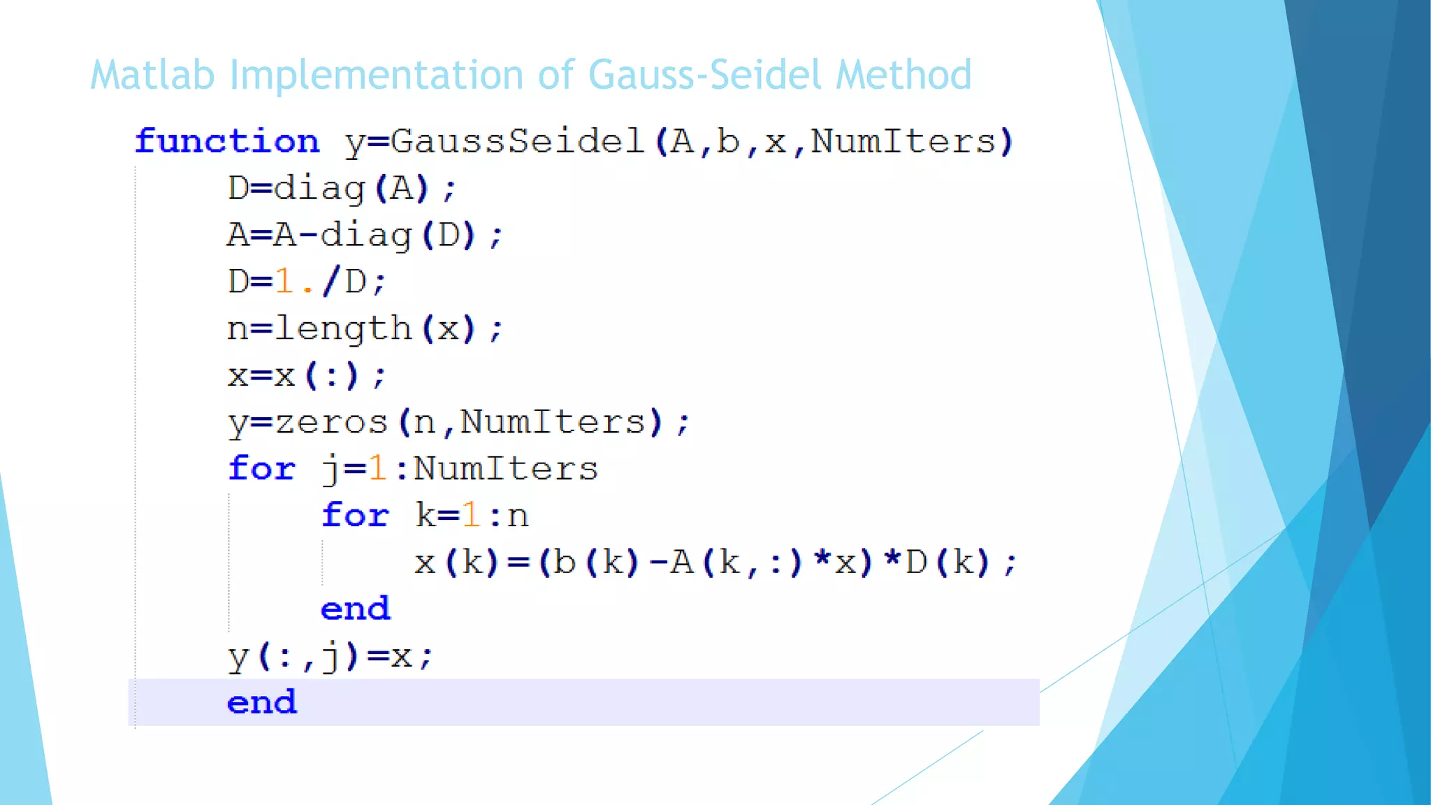
computing discrete
approximation of solution
of linear simultaneous
equation
JMHM Jayamaha
Content
 Linear Equations
 What is Linear Equations
 Method for solving the system of linear equations
 Direct Method
 Gauss Elimination method
 LU Decomposition
 Iterative method
 Jacobi's method
 Gauss Seidal method
Linear Equations
What is Linear Equations
 A linear equation is an algebraic equation in which each term is either
a constant or the product of a constant and (the first power of) a
single variable.
Two methods for solving the system of linear
equations
 Direct Method
 Solutions are obtained through a finite number of arithmetic operations
 Gauss Elimination method
 LU Decomposition
 Iterative Method:
 Solutions are obtained through a sequence of successive approximations
which converges to the required solution
 Jacobi's method
 Gauss Seidal method
GAUSS – ELIMINATION METHOD
Consider a system of 3 – equations with 3 – unknowns
)1(
3333232131
2323222121
1313212111








bxaxaxa
bxaxaxa
bxaxaxa
Form the augmented matrix from the given equations as










3333231
2232221
1131211
baaa
baaa
baaa



1
11
21
22operationrowtheUse R
a
a
RR 
1
11
31
33operationrowtheUse R
a
a
RR 
If a11  0
New augmented matrix will be










'''0
'''0
33332
22322
1131211
baa
baa
baaa



2
22
32
33
'
'
operationrowtheUse R
a
a
RR 
New augmented matrix will be










''''00
'''0
333
22322
1131211
ba
baa
baaa



If a22’  0
From the last matrix, the equations can be written as
''''
'''
3333
2323222
1313212111
bxa
bxaxa
bxaxaxa



Use back substitution to get the solution as
11
3132121
1
22
3232
2
33
3
3
,
'
''
,
''
''
a
xaxab
x
a
xab
x
a
b
x





Gauss Elimination method Matlab Implementation
function x = Gauss(A,b);
n = length(b); x = zeros(n,1);
for k=1:n-1 % forward elimination
for i=k+1:n
xmult = A(i,k)/A(k,k);
for j=k+1:n
A(i,j) = A(i,j)-xmult*A(k,j);
end
b(i) = b(i)-xmult*b(k);
end
end
% back substitution
x(n) = b(n)/A(n,n);
for i=n-1:-1:1
sum = b(i);
for j=i+1:n
sum = sum-A(i,j)*x(j);
end
x(i) = sum/A(i,i);
end
LU Decomposition
 Matrix A is decomposed into a product of a lower triangular
matrix L and an upper triangular matrix U, that is A = LU or































100
10
1
0
00
23
1312
333231
2221
11
333231
232221
131211
u
uu
lll
ll
l
aaa
aaa
aaa
Matrices L and U can be obtained by the following rule
1. Step 1: Obtain l11 = a11, l21 = a21, l31 = a31
11
13
13
11
12
12 ,Obtain:2Step.2
a
a
u
a
a
u 
3. Step 3: Obtain l22 = a22 – l21u12
 132123
22
23
1
Obtain:4Step.4 ula
l
u 
5. Step 5: Obtain l32 = a32 – l31u12
6. Step 6: Obtain l33 = a33 – l31u13 – l32u23
Once lower and upper triangular matrices are obtained the
solution of Ax = b can be obtained using the procedure
Ax = b  LUx = b
Let Ux = y
then
LUx = b  Ly = b
Steps to get the solution of linear equations
































3
2
1
3
2
1
333231
2221
11
0
00
b
b
b
y
y
y
lll
ll
l
bLy
 
 2321313
33
3
1212
22
2
11
1
1
1
and
1
,where
ylylb
l
y
ylb
l
y
l
b
y


By Forward substitution
































3
2
1
3
2
1
23
1312
100
10
1
Now
b
b
b
x
x
x
u
uu
bUx
31321211
3232233 ,where
xuxuyx
xuyxyx


By Backward substitution
Matlab Implementation for LU Decomposition
Iterative methods
The Jacobi Method
The Jacobi Method
 This method makes two assumptions
1. that the system given by has a unique solution
2. the coefficient matrix A has no zeros on its main diagonal
 To begin the Jacobi method, solve the first equation for x1 the second
equation for x2 and so on, as follows.
 Then make an initial approximation of the solution,
Algorithm
 Example
 To begin, write the system in the form
 Because you do not know the actual solution, choose
 as a convenient initial approximation. So, the first approximation is
 Continuing this procedure, you obtain the sequence of approximations shown
in Table
 Because the last two columns in Table are identical, you can conclude that to
three significant digits the solution is
Matlab Implementation for jacobi method
Iterative methods
The Gauss-Seidel Method
 Gauss-Seidel iteration is similar to Jacobi iteration, except that new
values for xi are used on the right-hand side of the equations as soon
as they become available.
 It improves upon the Jacobi method in two respects
 Convergence is quicker, since you benefit from the newer, more accurate
xi values earlier.
 Memory requirements are reduced by 50%, since you only need to keep
track of one set of xi values, not two sets.
Algorithm
 Example

 Step 1: reformat the equations, solving the first one for x1, the second for x2,
and the third for x3
 Step 2a: Substitute the initial guesses for xi into the right-hand side of the
first equation
 Step 2b: Substitute the new x1 value with the initial guess for x3 into the
second equation
 Step 2c: Substitute the new x1 and x2 values into the third equation
 Step 3, 4, · · · : Repeat step 2 and watch for the xi values to converge to an
exact solution.
Matlab Implementation of Gauss-Seidel Method
Summary
 Solution of linear simultaneous are discussed.
 Two methods
 Direct
 Gauss Elimination method
 LU Decomposition
 Iterative
 Jacobi's method
 Gauss Seidal method
References
 https://en.wikipedia.org/wiki/Linear_equation(2016-06-15)
 http://homel.vsb.cz/~dom033/predmety/parisLA/02_direct_methods.pdf
 Numerical computational methods by P.B Patill , U.P Verma
 http://college.cengage.com/mathematics/larson/elementary_linear/5e/stud
ents/ch08-10/chap_10_2.pdf
 http://ocw.usu.edu/Civil_and_Environmental_Engineering/Numerical_Method
s_in_Civil_Engineering/NonLinearEquationsMatlab.pdf
 http://people.whitman.edu/~hundledr/courses/M467/GaussSeidel.pdf

Linear and non linear equation

  • 1.
    computing discrete approximation ofsolution of linear simultaneous equation JMHM Jayamaha
  • 2.
    Content  Linear Equations What is Linear Equations  Method for solving the system of linear equations  Direct Method  Gauss Elimination method  LU Decomposition  Iterative method  Jacobi's method  Gauss Seidal method
  • 3.
  • 4.
    What is LinearEquations  A linear equation is an algebraic equation in which each term is either a constant or the product of a constant and (the first power of) a single variable.
  • 5.
    Two methods forsolving the system of linear equations  Direct Method  Solutions are obtained through a finite number of arithmetic operations  Gauss Elimination method  LU Decomposition  Iterative Method:  Solutions are obtained through a sequence of successive approximations which converges to the required solution  Jacobi's method  Gauss Seidal method
  • 6.
  • 7.
    GAUSS – ELIMINATIONMETHOD Consider a system of 3 – equations with 3 – unknowns )1( 3333232131 2323222121 1313212111         bxaxaxa bxaxaxa bxaxaxa
  • 8.
    Form the augmentedmatrix from the given equations as           3333231 2232221 1131211 baaa baaa baaa    1 11 21 22operationrowtheUse R a a RR  1 11 31 33operationrowtheUse R a a RR  If a11  0
  • 9.
    New augmented matrixwill be           '''0 '''0 33332 22322 1131211 baa baa baaa   
  • 10.
    2 22 32 33 ' ' operationrowtheUse R a a RR  Newaugmented matrix will be           ''''00 '''0 333 22322 1131211 ba baa baaa    If a22’  0
  • 11.
    From the lastmatrix, the equations can be written as '''' ''' 3333 2323222 1313212111 bxa bxaxa bxaxaxa   
  • 12.
    Use back substitutionto get the solution as 11 3132121 1 22 3232 2 33 3 3 , ' '' , '' '' a xaxab x a xab x a b x     
  • 13.
    Gauss Elimination methodMatlab Implementation function x = Gauss(A,b); n = length(b); x = zeros(n,1); for k=1:n-1 % forward elimination for i=k+1:n xmult = A(i,k)/A(k,k); for j=k+1:n A(i,j) = A(i,j)-xmult*A(k,j); end b(i) = b(i)-xmult*b(k); end end % back substitution x(n) = b(n)/A(n,n); for i=n-1:-1:1 sum = b(i); for j=i+1:n sum = sum-A(i,j)*x(j); end x(i) = sum/A(i,i); end
  • 14.
  • 15.
     Matrix Ais decomposed into a product of a lower triangular matrix L and an upper triangular matrix U, that is A = LU or                                100 10 1 0 00 23 1312 333231 2221 11 333231 232221 131211 u uu lll ll l aaa aaa aaa
  • 16.
    Matrices L andU can be obtained by the following rule 1. Step 1: Obtain l11 = a11, l21 = a21, l31 = a31 11 13 13 11 12 12 ,Obtain:2Step.2 a a u a a u  3. Step 3: Obtain l22 = a22 – l21u12  132123 22 23 1 Obtain:4Step.4 ula l u  5. Step 5: Obtain l32 = a32 – l31u12 6. Step 6: Obtain l33 = a33 – l31u13 – l32u23
  • 17.
    Once lower andupper triangular matrices are obtained the solution of Ax = b can be obtained using the procedure Ax = b  LUx = b Let Ux = y then LUx = b  Ly = b
  • 18.
    Steps to getthe solution of linear equations                                 3 2 1 3 2 1 333231 2221 11 0 00 b b b y y y lll ll l bLy    2321313 33 3 1212 22 2 11 1 1 1 and 1 ,where ylylb l y ylb l y l b y   By Forward substitution
  • 19.
  • 20.
    Matlab Implementation forLU Decomposition
  • 21.
  • 22.
    The Jacobi Method This method makes two assumptions 1. that the system given by has a unique solution 2. the coefficient matrix A has no zeros on its main diagonal
  • 23.
     To beginthe Jacobi method, solve the first equation for x1 the second equation for x2 and so on, as follows.  Then make an initial approximation of the solution,
  • 24.
  • 25.
  • 26.
     To begin,write the system in the form  Because you do not know the actual solution, choose
  • 27.
     as aconvenient initial approximation. So, the first approximation is  Continuing this procedure, you obtain the sequence of approximations shown in Table
  • 28.
     Because thelast two columns in Table are identical, you can conclude that to three significant digits the solution is
  • 29.
  • 30.
  • 31.
     Gauss-Seidel iterationis similar to Jacobi iteration, except that new values for xi are used on the right-hand side of the equations as soon as they become available.  It improves upon the Jacobi method in two respects  Convergence is quicker, since you benefit from the newer, more accurate xi values earlier.  Memory requirements are reduced by 50%, since you only need to keep track of one set of xi values, not two sets.
  • 32.
  • 33.
  • 34.
     Step 1:reformat the equations, solving the first one for x1, the second for x2, and the third for x3
  • 35.
     Step 2a:Substitute the initial guesses for xi into the right-hand side of the first equation  Step 2b: Substitute the new x1 value with the initial guess for x3 into the second equation  Step 2c: Substitute the new x1 and x2 values into the third equation
  • 36.
     Step 3,4, · · · : Repeat step 2 and watch for the xi values to converge to an exact solution.
  • 37.
    Matlab Implementation ofGauss-Seidel Method
  • 38.
    Summary  Solution oflinear simultaneous are discussed.  Two methods  Direct  Gauss Elimination method  LU Decomposition  Iterative  Jacobi's method  Gauss Seidal method
  • 39.
    References  https://en.wikipedia.org/wiki/Linear_equation(2016-06-15)  http://homel.vsb.cz/~dom033/predmety/parisLA/02_direct_methods.pdf Numerical computational methods by P.B Patill , U.P Verma  http://college.cengage.com/mathematics/larson/elementary_linear/5e/stud ents/ch08-10/chap_10_2.pdf  http://ocw.usu.edu/Civil_and_Environmental_Engineering/Numerical_Method s_in_Civil_Engineering/NonLinearEquationsMatlab.pdf  http://people.whitman.edu/~hundledr/courses/M467/GaussSeidel.pdf

Editor's Notes

  • #5 A linear equation is an algebraic equation in which each term is either a constant or the product of a constant and (the first power of) a single variable
  • #8 It is a direct method for finding the solution of a system of linear equations and is based on the principle of elimination. where aij(1)’s (i, j = 1, 2, 3) are the coefficient of unknowns and bi(1)’s (i = 1, 2, 3) are prescribed constants
  • #23 If any of the diagonal entries a11, a22, . . . , ann are zero, then rows or columns must be interchanged to obtain a coefficient matrix that has nonzero entries on the main diagonal.
  • #24 To begin the Jacobi method, solve the first equation for x1 the second equation for x2 and so on, as follows. Initial Approximation and substitute these values of xi into the right-hand side of the rewritten equations to obtain the first approximation. After this procedure has been completed, one iteration has been performed.
  • #26 In the same way, the second approximation is formed by substituting the first approximation’s x-values into the right-hand side of the rewritten equations. By repeated iterations, you will form a sequence of approximations that often converges to the actual solution.
  • #31 Iterative methods provide an alternative approach that an iterative methods starts with an approximate solution , and uses it by means of a recrurrence fomula to provie another approximate solution ; by repeatedly applying the formula, a sequence of solution is abtained with ( under suitable conditions)( converges to the exact solution . Iterative methods have the advantages of simplicity of operation and ease of implementation of computers. And they are realativelyi insensitive to propagation of errors; they would be used in preference to direct methods for solving lenear systems involving several handred variables. Particularly , if many of the coefficients were zero . Systems of over 100000 variable have more variables are difficult or impossible to solve by direct methods.