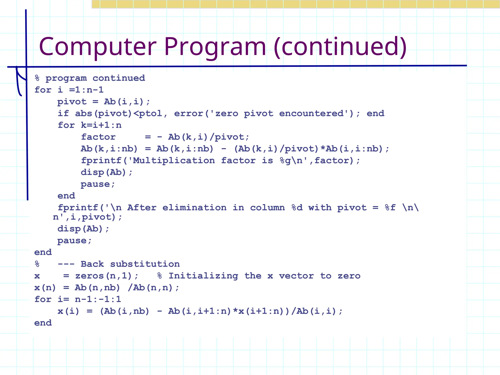
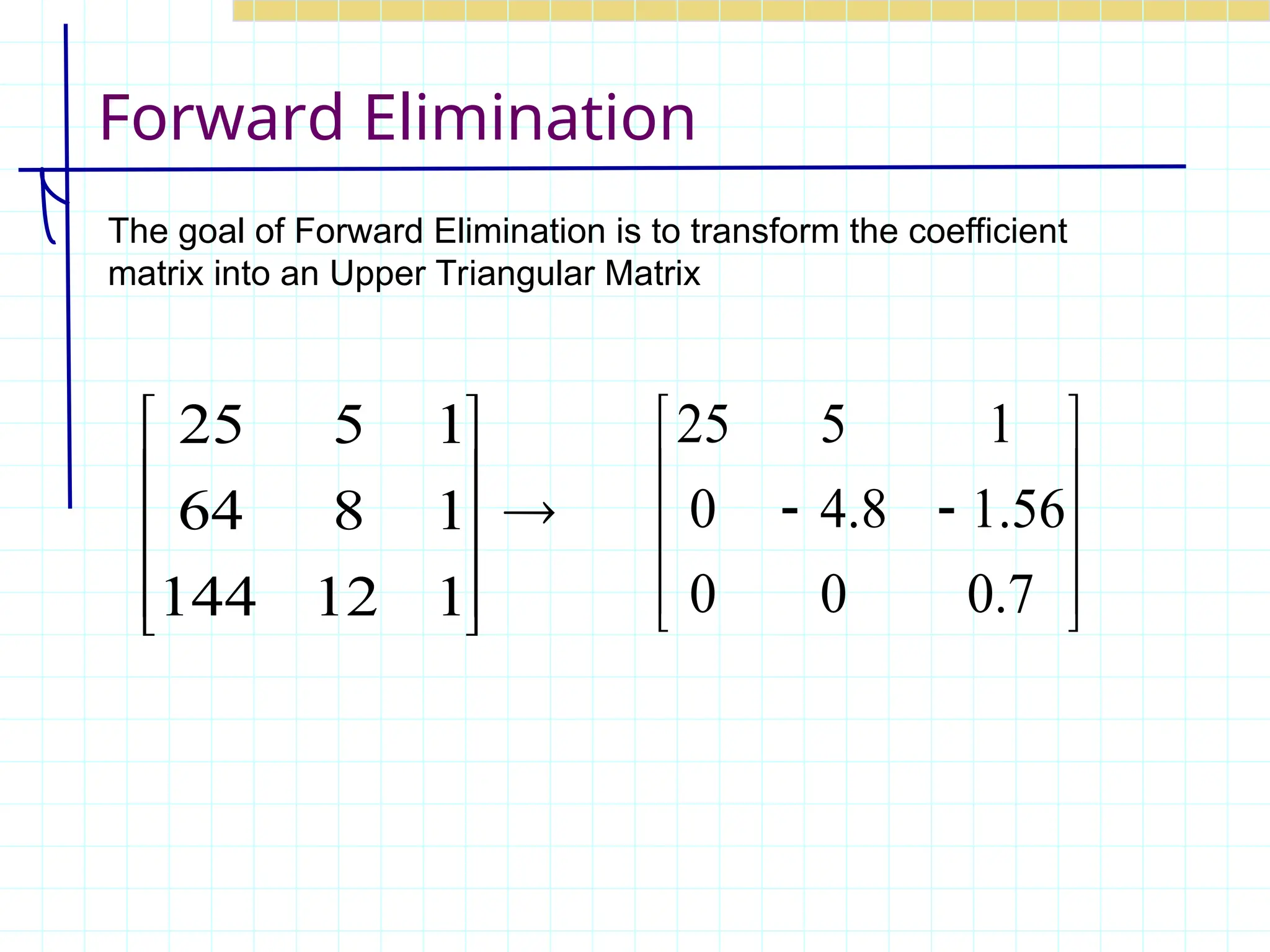
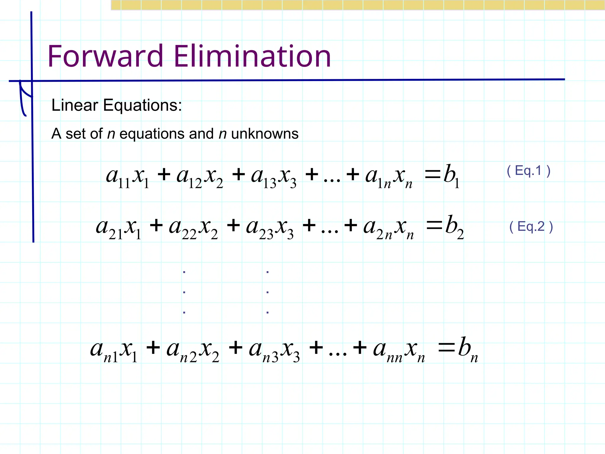
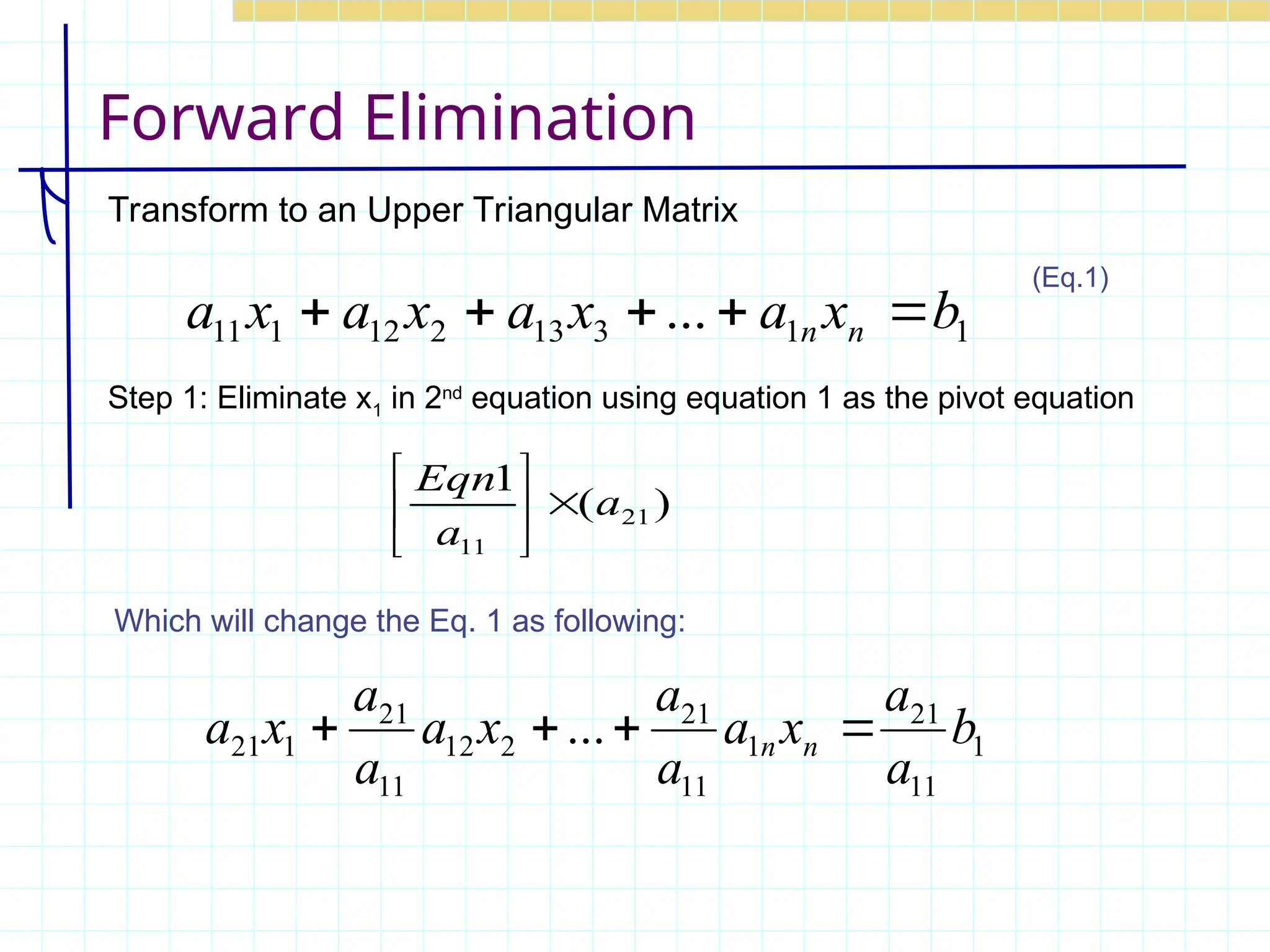
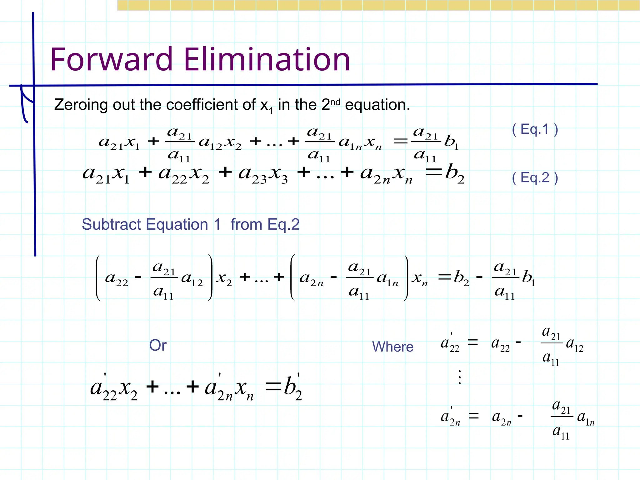
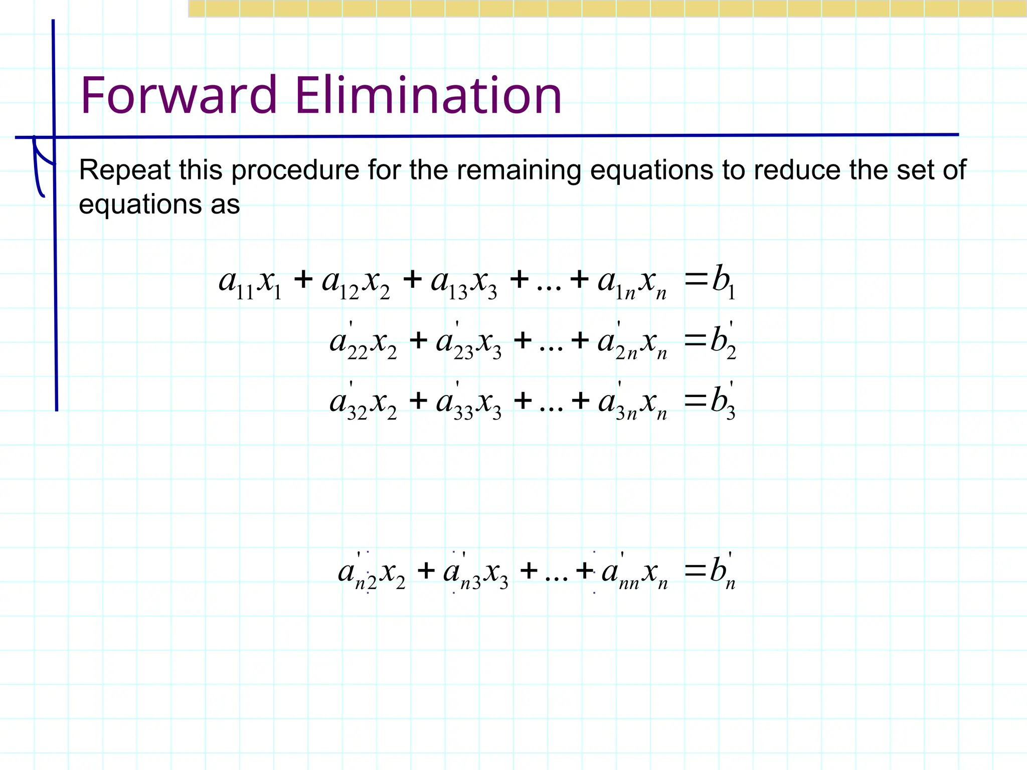
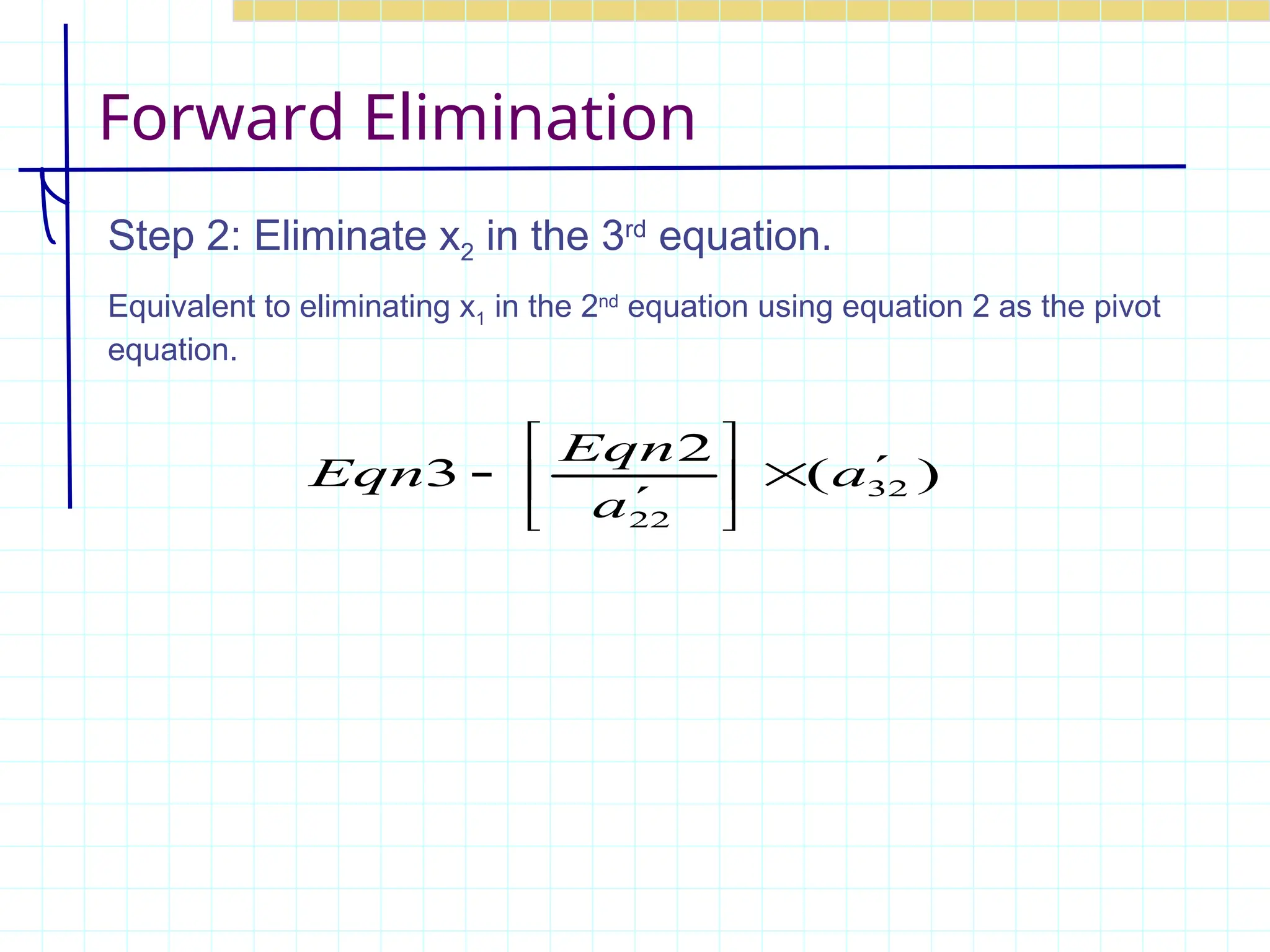
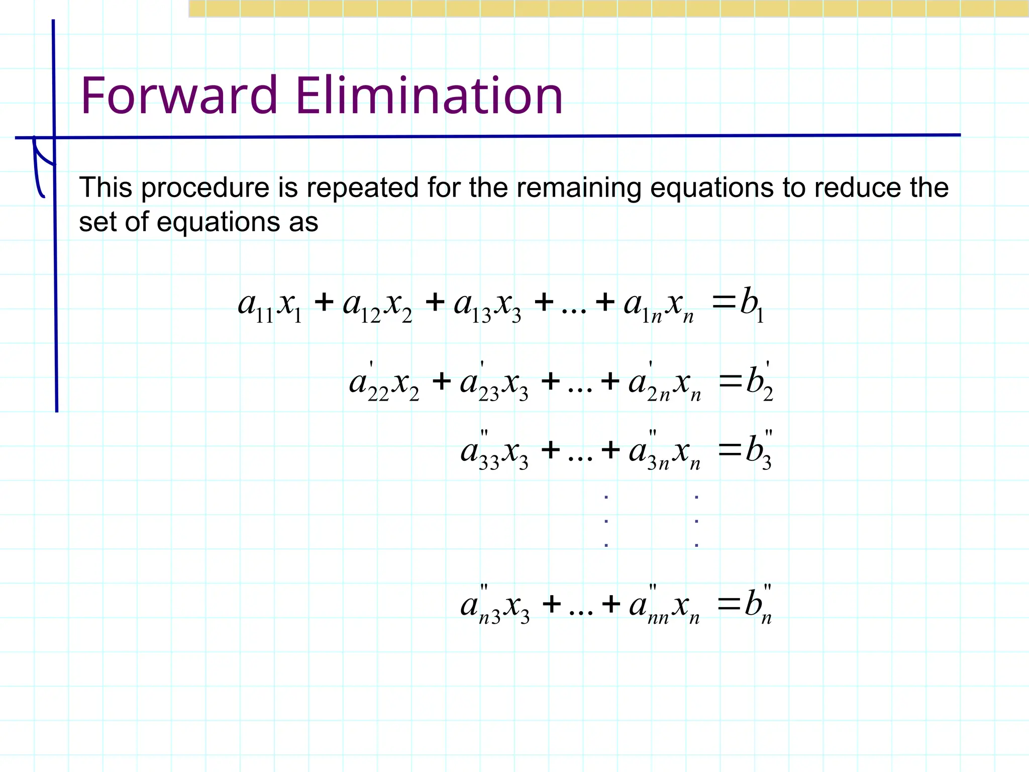
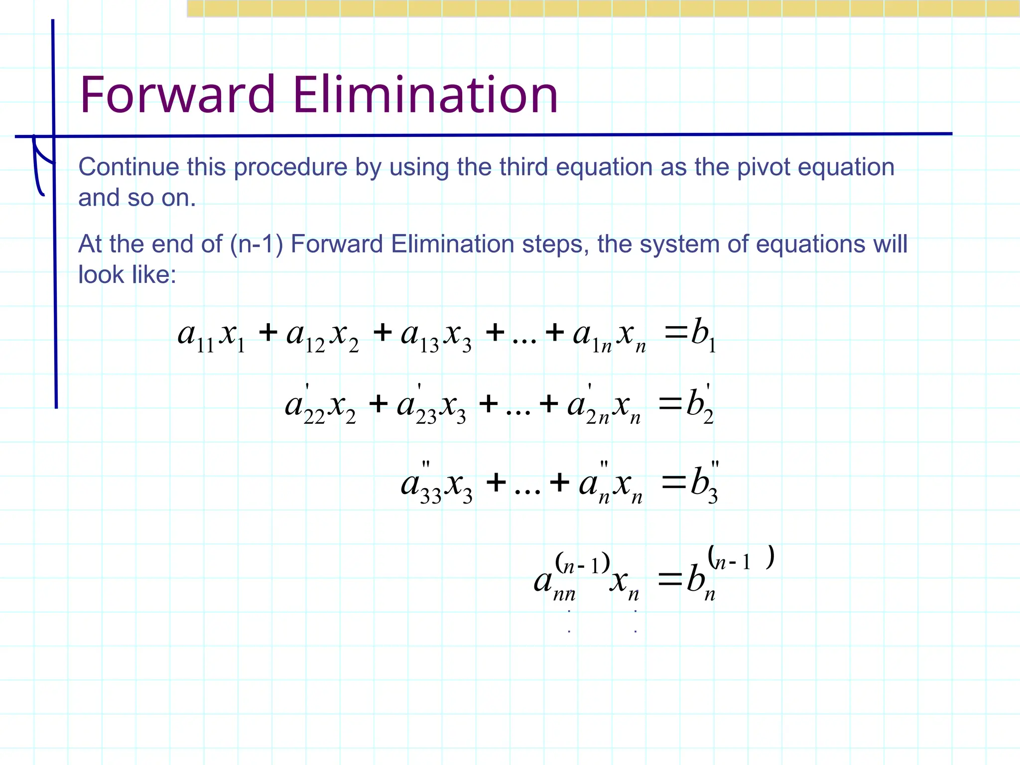
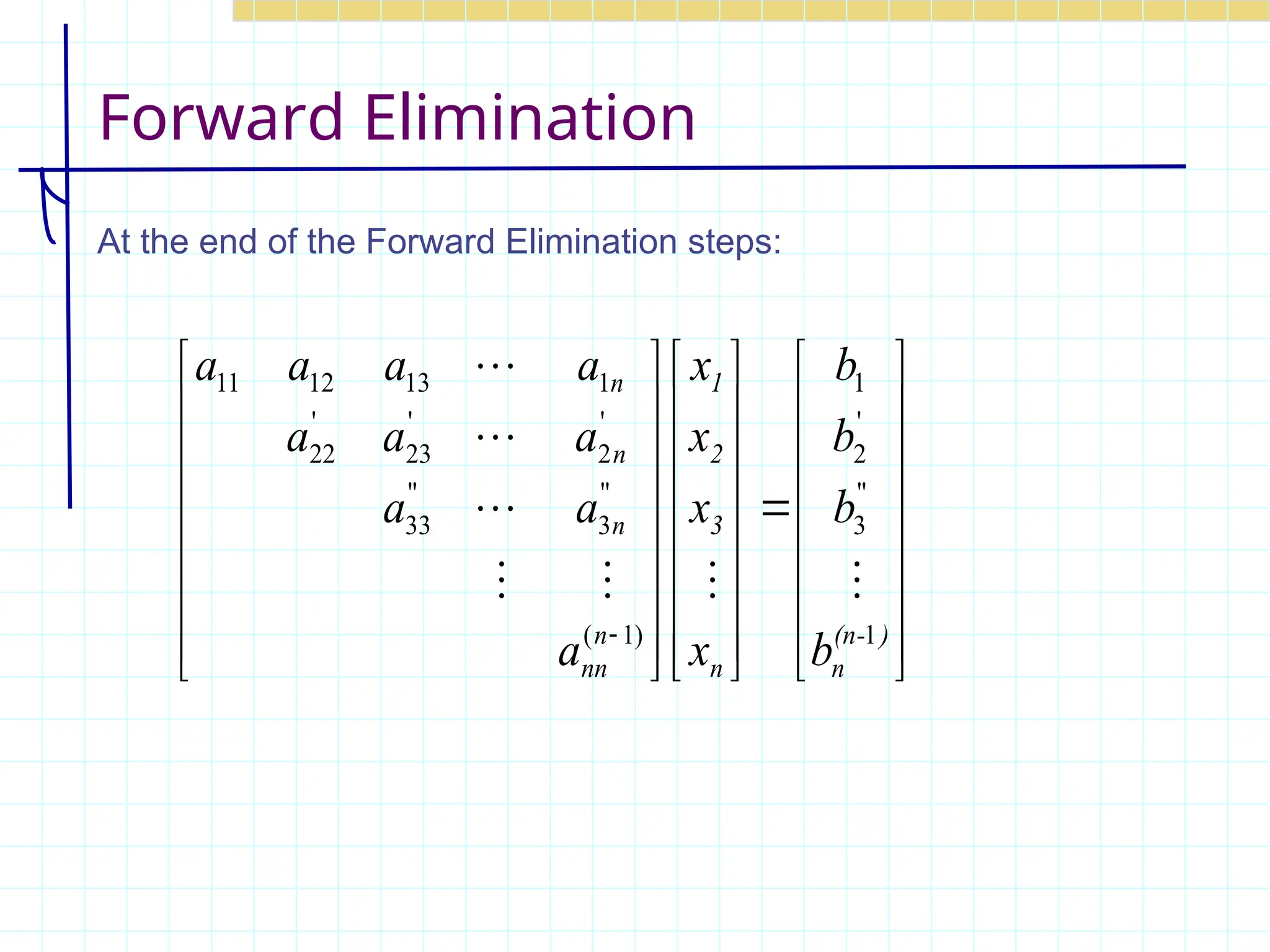
The document provides an overview of Gaussian elimination, a numerical method for solving simultaneous linear equations represented in matrix form. It explains concepts such as matrix rank, consistency of equations, and details the elimination and back substitution processes involved in solving the equations. Examples illustrate the steps taken to achieve solutions through this method.

1. Simultaneous Linear Equations
Topic: Gaussian Elimination
Dr. Nasir M Mirza
Numerical Methods
Numerical Methods
Email: nasirmm@yahoo.com

2. Gaussian Elimination

3. Basic Principles
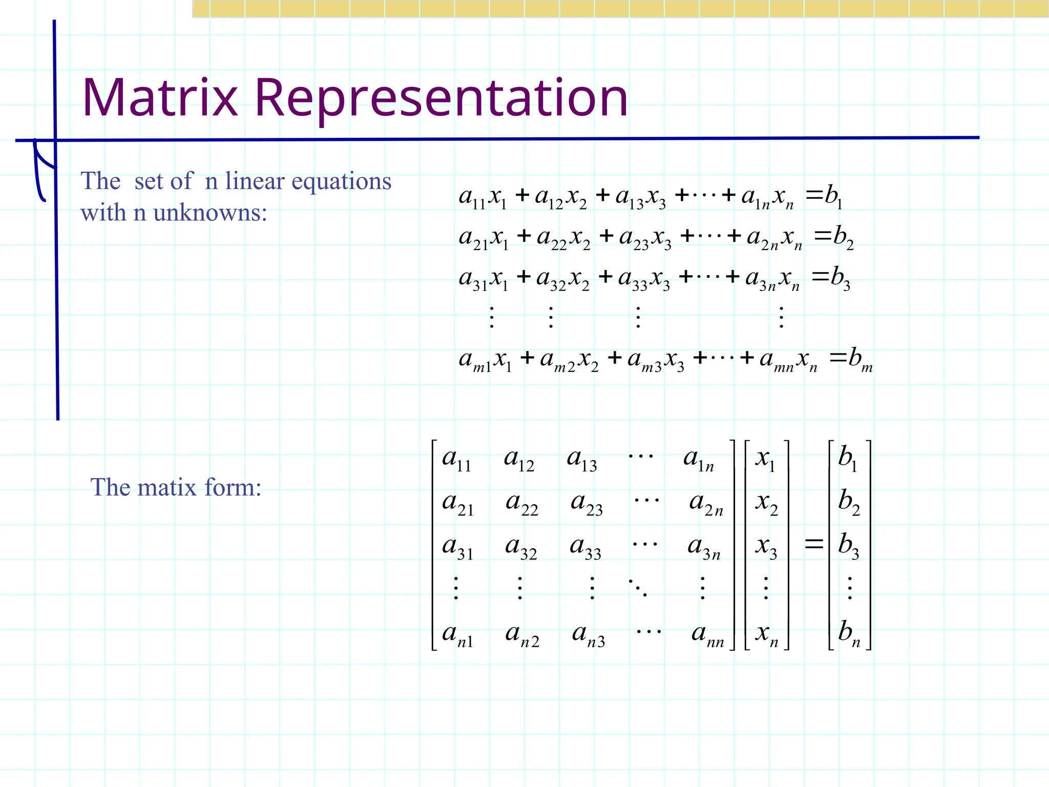
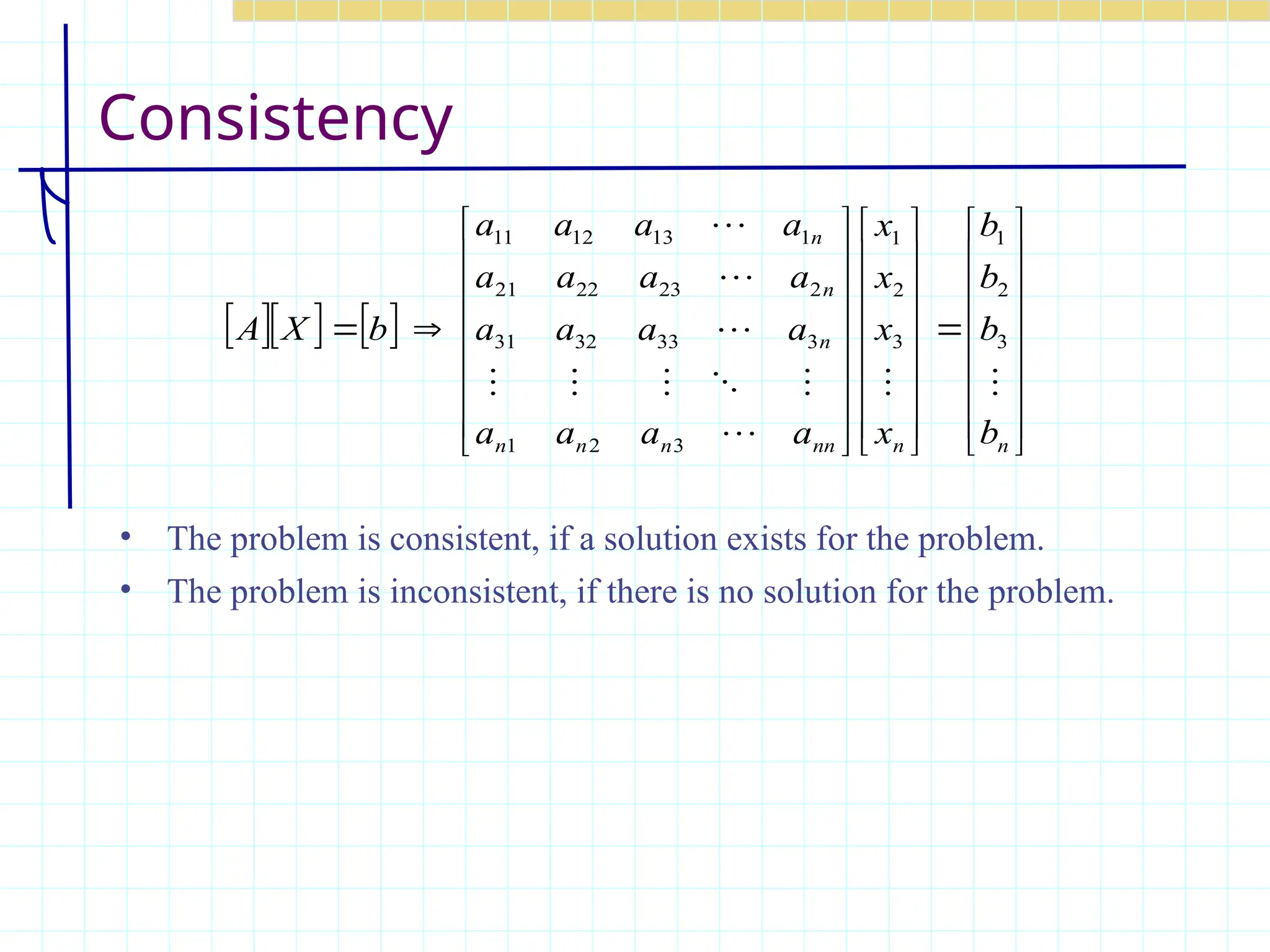
• The general description of a set of linear equations in the matrix
form: [A][X] = [B]
• Where, [A] is ( m x n ) matrix, the [X] is a ( n x 1 ) vector, and
the [B] is a (m x 1 ) vector.
• Where m in no. of rows and n is no. of columns.
• How we solve such a system:
• Write the equations in natural form
• Identify unknowns and order them
• Isolate unknowns
• Write equations in matrix form

4. Types of Matrix Formulation
If m = n The solution of [A]{x} ={b} with n unknowns and m(n) equations
If m > n The system is overdetermined system (Least Square Problems)
If m < n The system is underdetermined system (Optimization Problems)
m
n
mn
m
m
m
n
n
n
n
n
n
b
x
a
x
a
x
a
x
a
b
x
a
x
a
x
a
x
a
b
x
a
x
a
x
a
x
a
b
x
a
x
a
x
a
x
a




























3
3
2
2
1
1
3
3
3
33
2
32
1
31
2
2
3
23
2
22
1
21
1
1
3
13
2
12
1
11
Suppose we have an ( m x n ) Array

5. Matrix Representation

















































n
n
nn
n
n
n
n
n
n
b
b
b
b
x
x
x
x
a
a
a
a
a
a
a
a
a
a
a
a
a
a
a
a











3
2
1
3
2
1
3
2
1
3
33
32
31
2
23
22
21
1
13
12
11
m
n
mn
m
m
m
n
n
n
n
n
n
b
x
a
x
a
x
a
x
a
b
x
a
x
a
x
a
x
a
b
x
a
x
a
x
a
x
a
b
x
a
x
a
x
a
x
a




























3
3
2
2
1
1
3
3
3
33
2
32
1
31
2
2
3
23
2
22
1
21
1
1
3
13
2
12
1
11
The set of n linear equations
with n unknowns:
The matix form:

6. Consistency
    



















































n
n
nn
n
n
n
n
n
n
b
b
b
b
x
x
x
x
a
a
a
a
a
a
a
a
a
a
a
a
a
a
a
a
b
X
A











3
2
1
3
2
1
3
2
1
3
33
32
31
2
23
22
21
1
13
12
11
• The problem is consistent, if a solution exists for the problem.
• The problem is inconsistent, if there is no solution for the problem.

7. Rank of Matrix
Rank of a matrix is the number of linearly
independent column vectors in the matrix.
For n x n matrix, A:
• If rank(A) = n and is consistent, A has an unique
solution exists
• If rank(A) = n and is inconsistent, A has no solution
exists
• If rank(A) < n and system is consistent, A has an
infinite number of solutions

8. Matrix
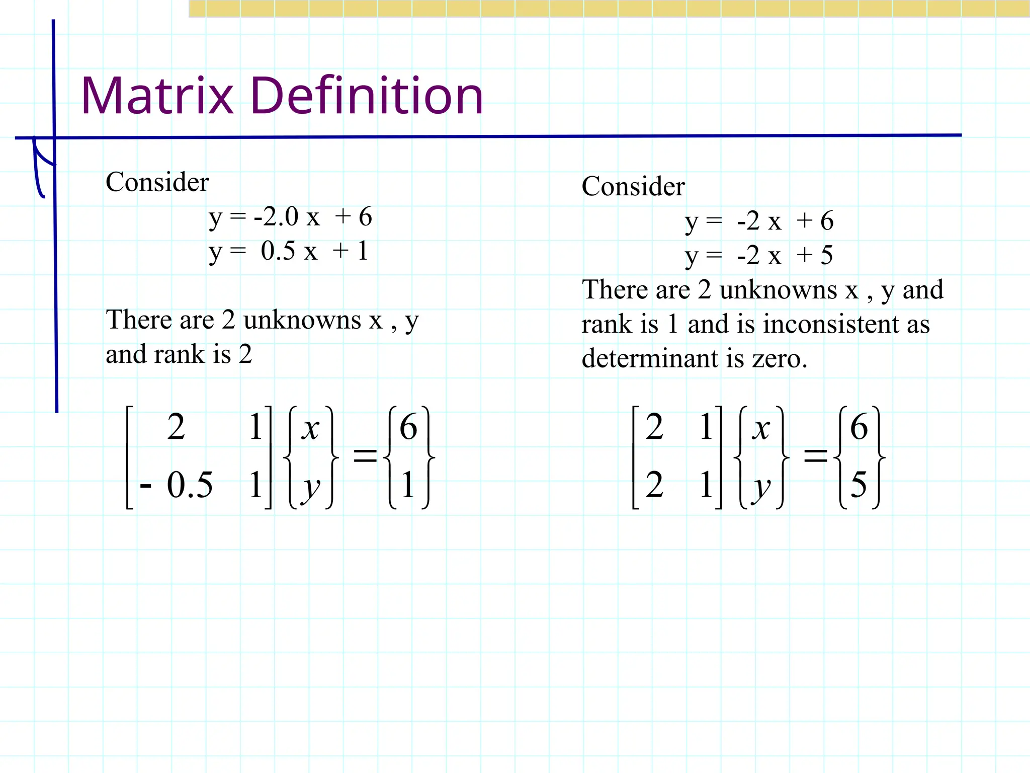
For an n x n system, rank(A) = n automatically
guarantees
that the system is consistent.
• The columns of A are linearly independent
• The rows of A are linearly independent
• rank(A) = n
• det(A) != 0
• A-1
exists;
• The solution to [A]{x} ={b} exist and is unique.

9. Matrix Definition



















 1
6
1
5
.
0
1
2
y
x



















5
6
1
2
1
2
y
x
Consider
y = -2.0 x + 6
y = 0.5 x + 1
There are 2 unknowns x , y
and rank is 2
Consider
y = -2 x + 6
y = -2 x + 5
There are 2 unknowns x , y and
rank is 1 and is inconsistent as
determinant is zero.

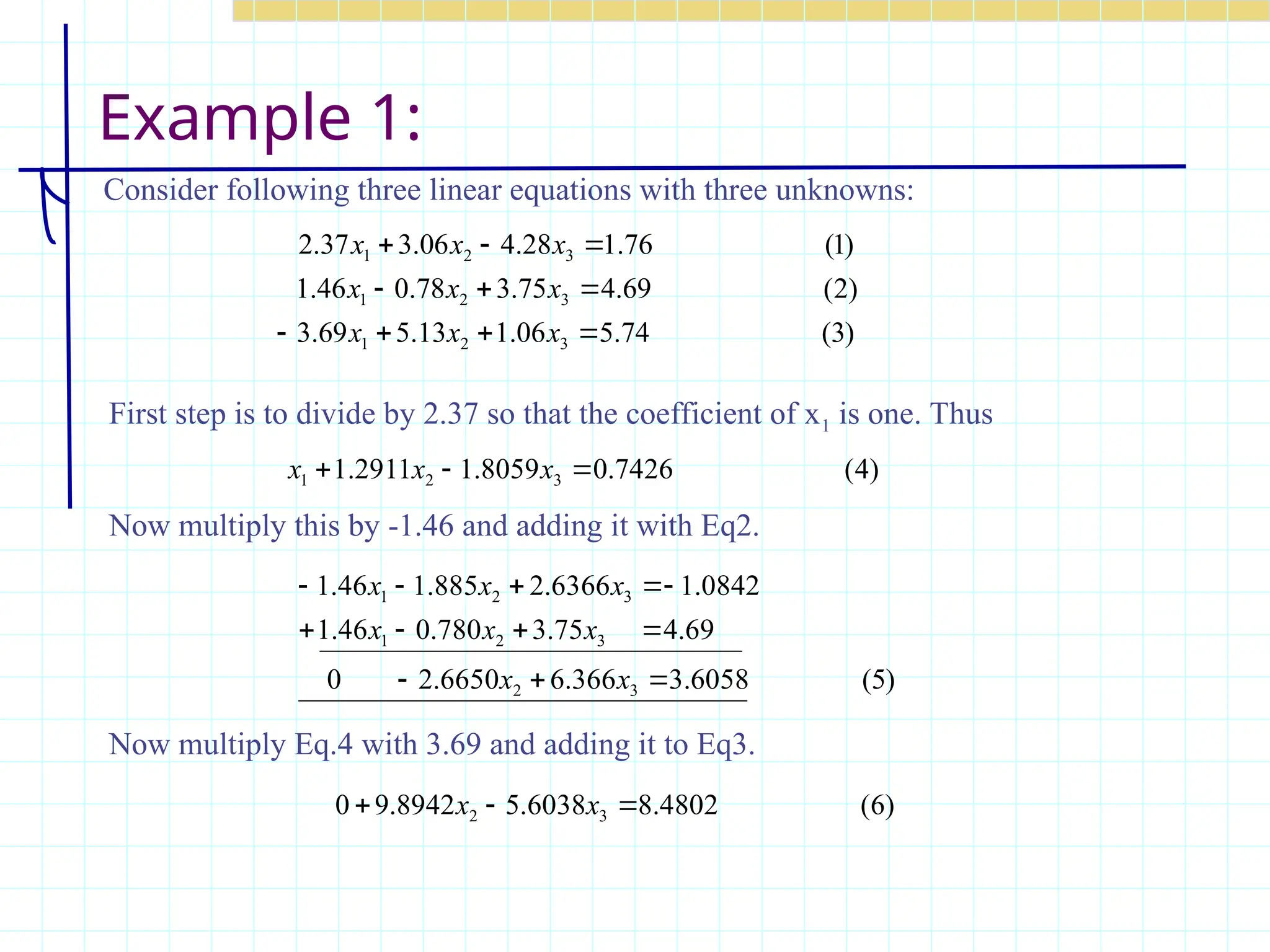
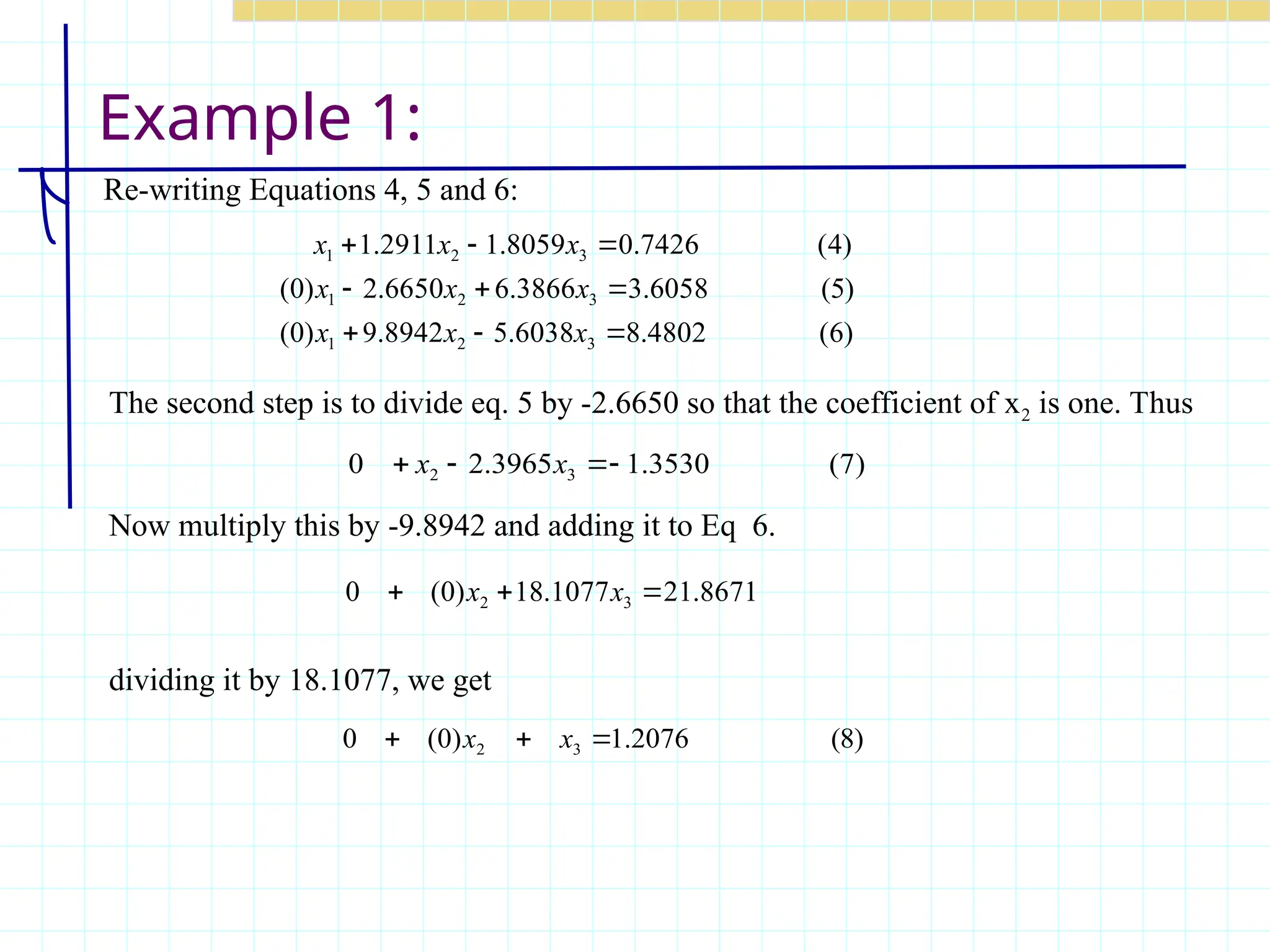
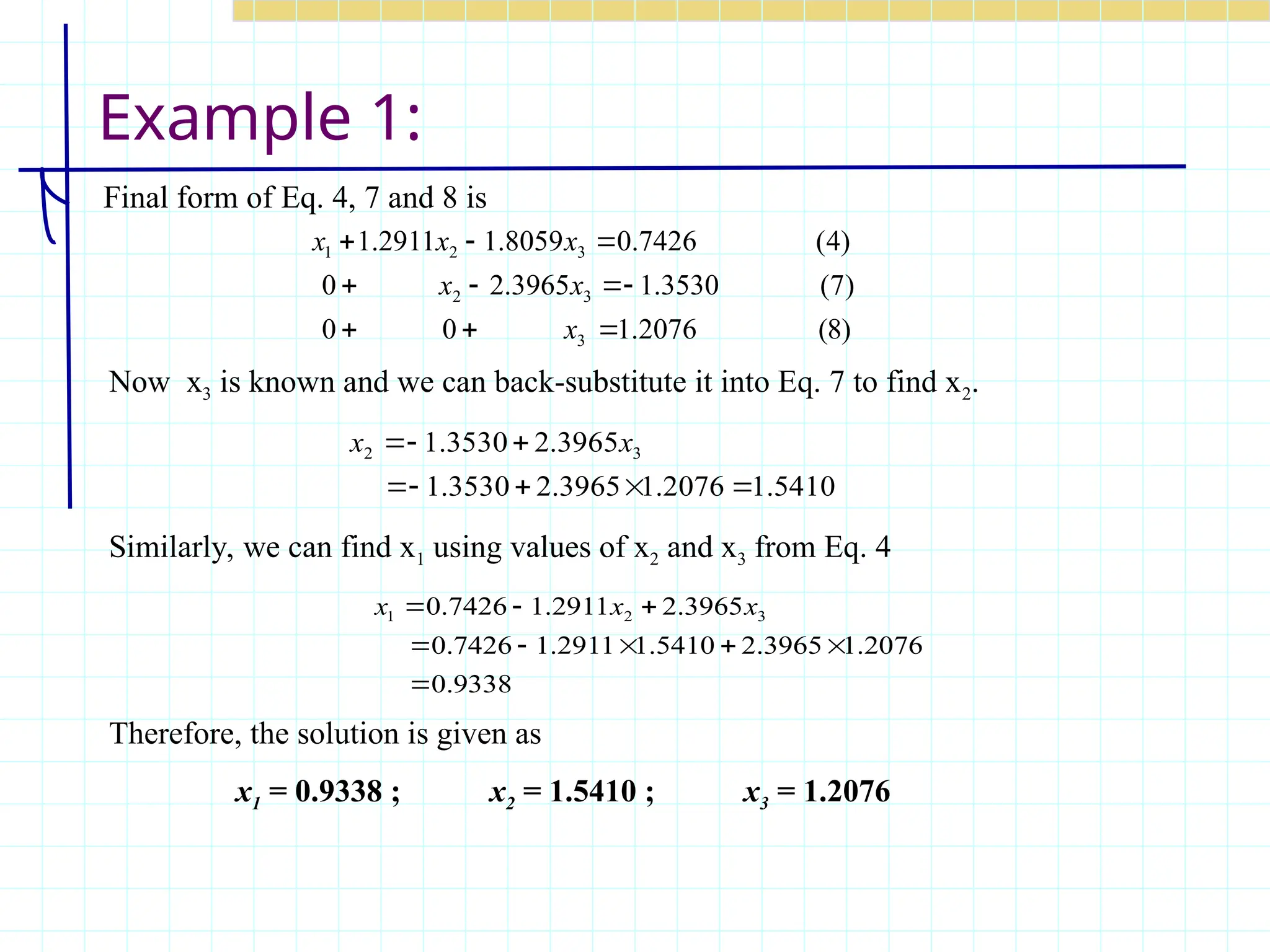
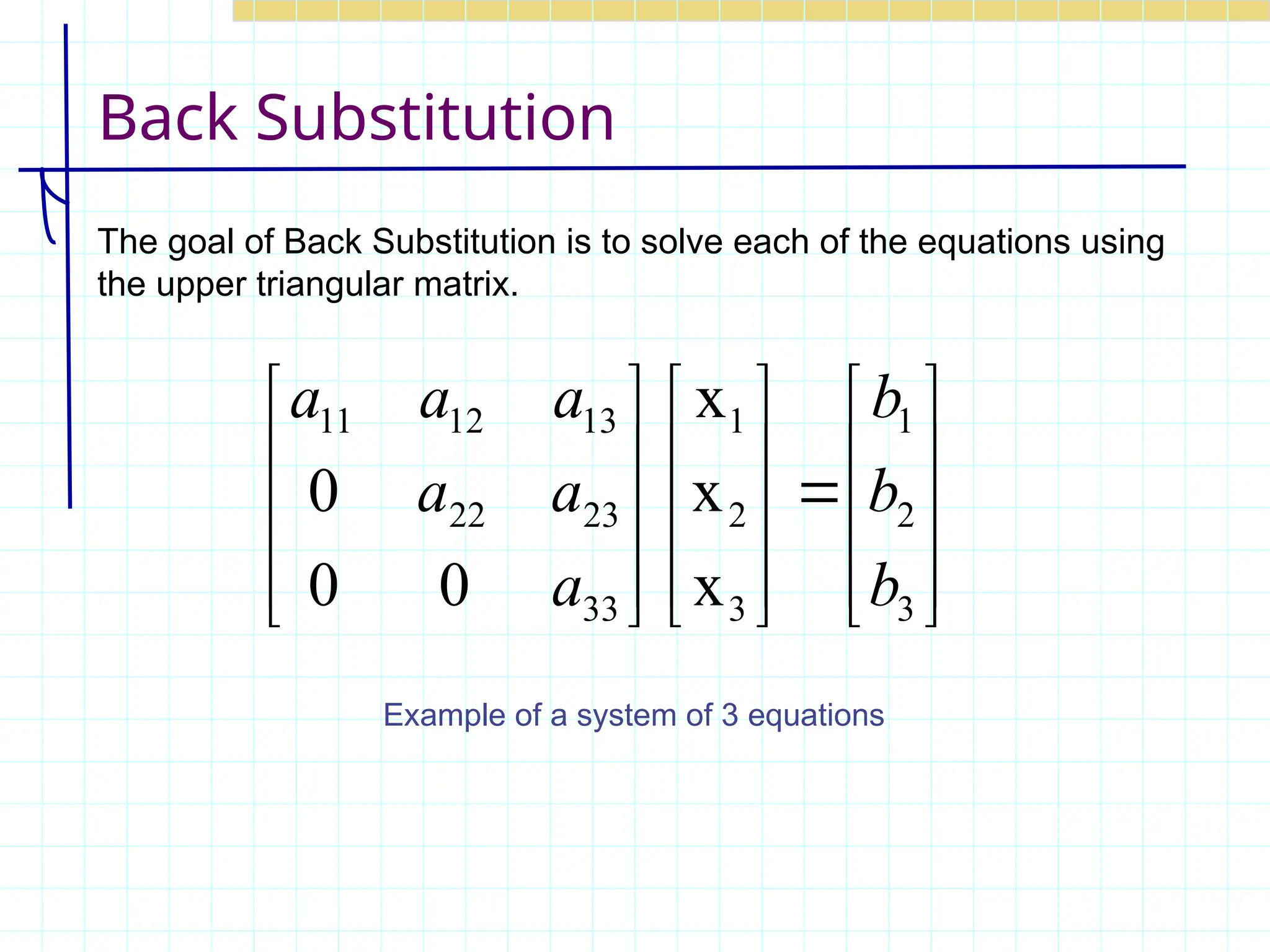
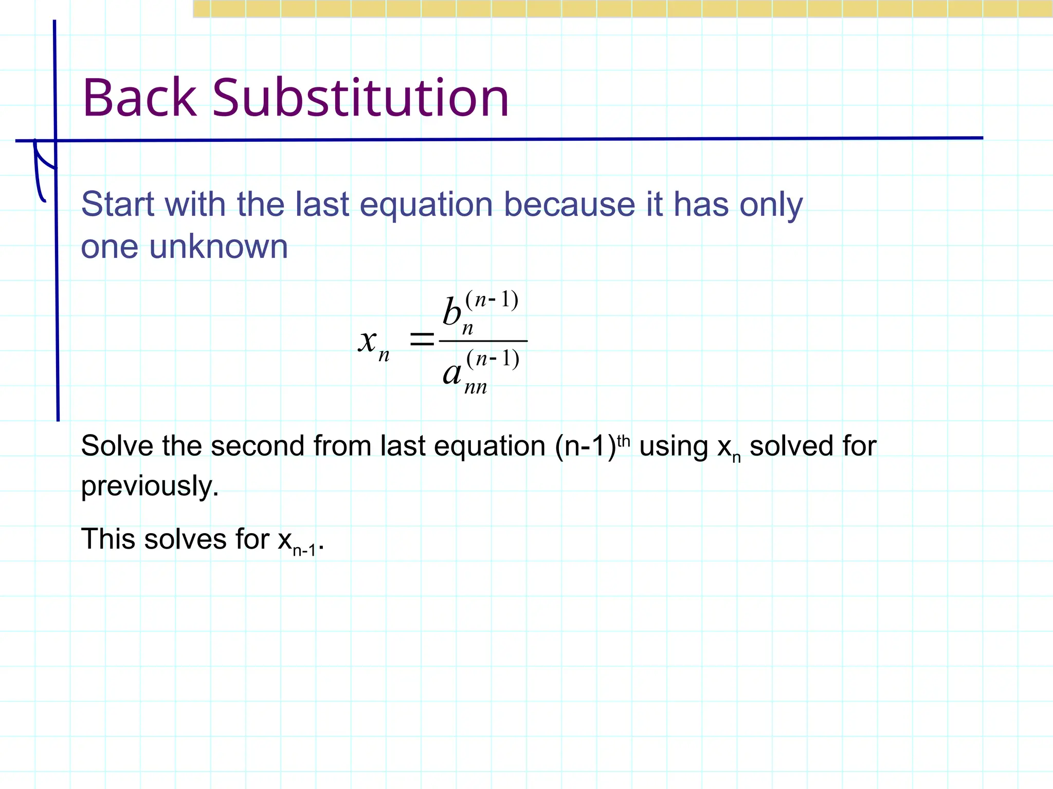
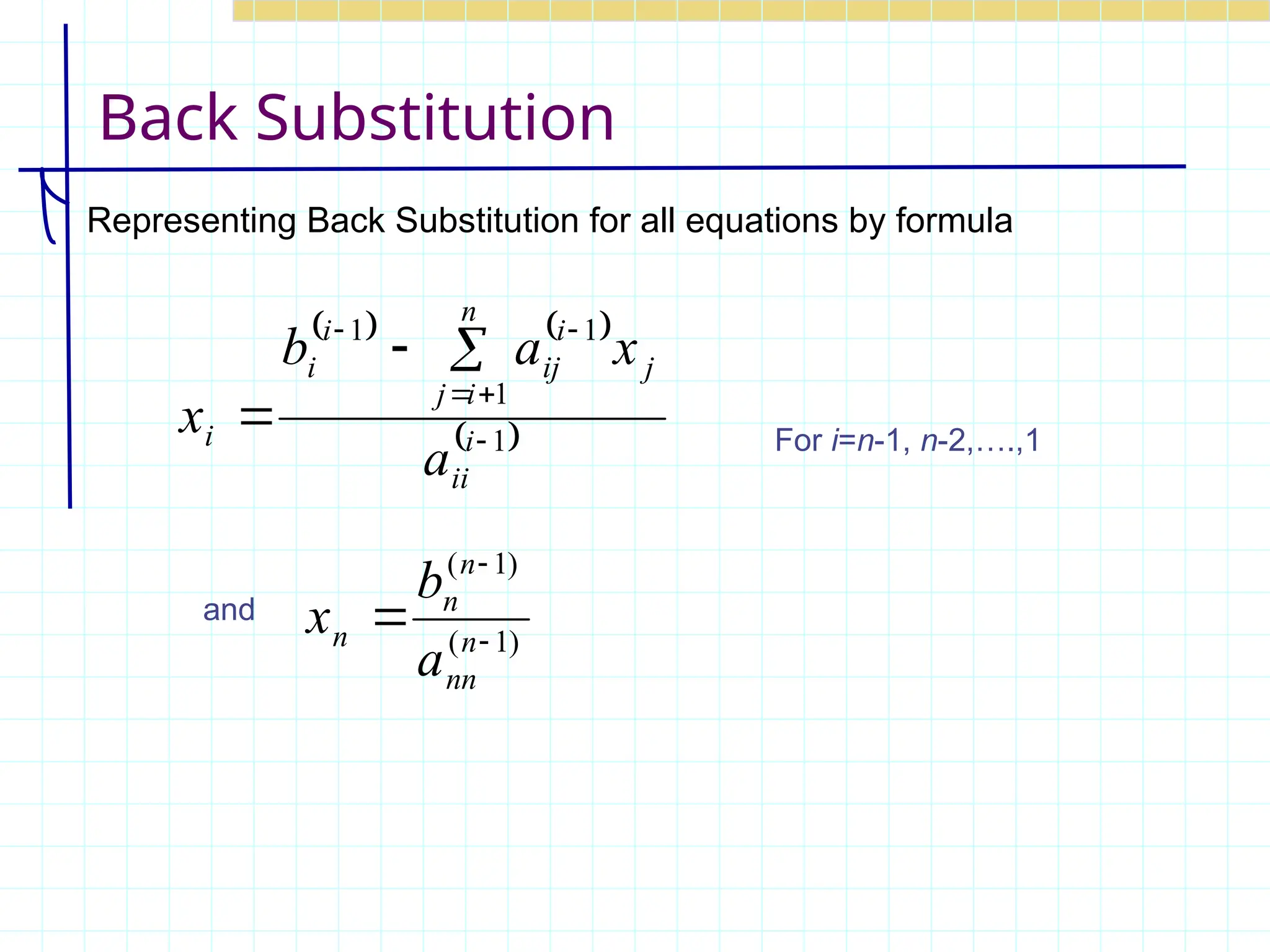
10. Gaussian Elimination
Gaussian Elimination is one of the most popular techniques for
solving simultaneous linear equations of the form: [A][X] =[b]
The method consists of 2 steps
1. Forward Elimination of Unknowns.
2. Back Substitution
Let us learn the method first by examples:
m
n
mn
m
m
m
n
n
n
n
n
n
b
x
a
x
a
x
a
x
a
b
x
a
x
a
x
a
x
a
b
x
a
x
a
x
a
x
a
b
x
a
x
a
x
a
x
a




























3
3
2
2
1
1
3
3
3
33
2
32
1
31
2
2
3
23
2
22
1
21
1
1
3
13
2
12
1
11

11. Example 1:
Consider following three linear equations with three unknowns:
)
3
(
74
.
5
06
.
1
13
.
5
69
.
3
)
2
(
69
.
4
75
.
3
78
.
0
46
.
1
)
1
(
76
.
1
28
.
4
06
.
3
37
.
2
3
2
1
3
2
1
3
2
1










x
x
x
x
x
x
x
x
x
)
4
(
7426
.
0
8059
.
1
2911
.
1 3
2
1 

 x
x
x
)
5
(
6058
.
3
366
.
6
6650
.
2
0
69
.
4
75
.
3
780
.
0
46
.
1
0842
.
1
6366
.
2
885
.
1
46
.
1
3
2
3
2
1
3
2
1












x
x
x
x
x
x
x
x
First step is to divide by 2.37 so that the coefficient of x1 is one. Thus
Now multiply this by -1.46 and adding it with Eq2.
)
6
(
4802
.
8
6038
.
5
8942
.
9
0 3
2 

 x
x
Now multiply Eq.4 with 3.69 and adding it to Eq3.

12. Example 1:
Re-writing Equations 4, 5 and 6:
)
6
(
4802
.
8
6038
.
5
8942
.
9
)
0
(
)
5
(
6058
.
3
3866
.
6
6650
.
2
)
0
(
)
4
(
7426
.
0
8059
.
1
2911
.
1
3
2
1
3
2
1
3
2
1









x
x
x
x
x
x
x
x
x
)
7
(
3530
.
1
3965
.
2
0 3
2 


 x
x
8671
.
21
1077
.
18
)
0
(
0 3
2 

 x
x
The second step is to divide eq. 5 by -2.6650 so that the coefficient of x2 is one. Thus
Now multiply this by -9.8942 and adding it to Eq 6.
dividing it by 18.1077, we get
)
8
(
2076
.
1
)
0
(
0 3
2 

 x
x

13. Example 1:
Final form of Eq. 4, 7 and 8 is
)
8
(
2076
.
1
0
0
)
7
(
3530
.
1
3965
.
2
0
)
4
(
7426
.
0
8059
.
1
2911
.
1
3
3
2
3
2
1










x
x
x
x
x
x
5410
.
1
2076
.
1
3965
.
2
3530
.
1
3965
.
2
3530
.
1 3
2







 x
x
Now x3 is known and we can back-substitute it into Eq. 7 to find x2.
Similarly, we can find x1 using values of x2 and x3 from Eq. 4
Therefore, the solution is given as
x1 = 0.9338 ; x2 = 1.5410 ; x3 = 1.2076
9338
.
0
2076
.
1
3965
.
2
5410
.
1
2911
.
1
7426
.
0
3965
.
2
2911
.
1
7426
.
0 3
2
1








 x
x
x

14. Forward Elimination
The goal of Forward Elimination is to transform the coefficient
matrix into an Upper Triangular Matrix
7
.
0
0
0
56
.
1
8
.
4
0
1
5
25























1
12
144
1
8
64
1
5
25

15. Forward Elimination
Linear Equations:
A set of n equations and n unknowns
1
1
3
13
2
12
1
11 ... b
x
a
x
a
x
a
x
a n
n 




2
2
3
23
2
22
1
21 ... b
x
a
x
a
x
a
x
a n
n 




n
n
nn
n
n
n b
x
a
x
a
x
a
x
a 



 ...
3
3
2
2
1
1
. .
. .
. .
( Eq.1 )
( Eq.2 )

16. Forward Elimination
Transform to an Upper Triangular Matrix
Step 1: Eliminate x1 in 2nd
equation using equation 1 as the pivot equation
)
(
1
21
11
a
a
Eqn







Which will change the Eq. 1 as following:
1
11
21
1
11
21
2
12
11
21
1
21 ... b
a
a
x
a
a
a
x
a
a
a
x
a n
n 



1
1
3
13
2
12
1
11 ... b
x
a
x
a
x
a
x
a n
n 




(Eq.1)

17. Forward Elimination
Zeroing out the coefficient of x1 in the 2nd
equation.
Subtract Equation 1 from Eq.2
1
11
21
2
1
11
21
2
2
12
11
21
22 ... b
a
a
b
x
a
a
a
a
x
a
a
a
a n
n
n 





















'
2
'
2
2
'
22 ... b
x
a
x
a n
n 


n
n
n a
a
a
a
a
a
a
a
a
a
1
11
21
2
'
2
12
11
21
22
'
22





Or
1
11
21
1
11
21
2
12
11
21
1
21 ... b
a
a
x
a
a
a
x
a
a
a
x
a n
n 



Where
2
2
3
23
2
22
1
21 ... b
x
a
x
a
x
a
x
a n
n 



 ( Eq.2 )
( Eq.1 )

18. Forward Elimination
Repeat this procedure for the remaining equations to reduce the set of
equations as
1
1
3
13
2
12
1
11 ... b
x
a
x
a
x
a
x
a n
n 




'
2
'
2
3
'
23
2
'
22 ... b
x
a
x
a
x
a n
n 



'
3
'
3
3
'
33
2
'
32 ... b
x
a
x
a
x
a n
n 



'
'
3
'
3
2
'
2 ... n
n
nn
n
n b
x
a
x
a
x
a 



. . .
. . .
. . .

19. Forward Elimination
Step 2: Eliminate x2 in the 3rd
equation.
Equivalent to eliminating x1 in the 2nd
equation using equation 2 as the pivot
equation.
)
(
2
3 32
22
a
a
Eqn
Eqn 










20. Forward Elimination
This procedure is repeated for the remaining equations to reduce the
set of equations as
1
1
3
13
2
12
1
11 ... b
x
a
x
a
x
a
x
a n
n 




'
2
'
2
3
'
23
2
'
22 ... b
x
a
x
a
x
a n
n 



"
3
"
3
3
"
33 ... b
x
a
x
a n
n 


"
"
3
"
3 ... n
n
nn
n b
x
a
x
a 


. .
. .
. .

21. Forward Elimination
Continue this procedure by using the third equation as the pivot equation
and so on.
At the end of (n-1) Forward Elimination steps, the system of equations will
look like:
'
2
'
2
3
'
23
2
'
22 ... b
x
a
x
a
x
a n
n 



"
3
"
3
"
33 ... b
x
a
x
a n
n 


   
1
1 


n
n
n
n
nn b
x
a . .
. .
. .
1
1
3
13
2
12
1
11 ... b
x
a
x
a
x
a
x
a n
n 





22. Forward Elimination
At the end of the Forward Elimination steps:

















































 )
-
(n
n
n
3
2
1
n
nn
n
n
n
b
b
b
b
x
x
x
x
a
a
a
a
a
a
a
a
a
a
1
"
3
'
2
1
)
1
(
"
3
"
33
'
2
'
23
'
22
1
13
12
11








23. Back Substitution
The goal of Back Substitution is to solve each of the equations using
the upper triangular matrix.































3
2
1
3
2
1
33
23
22
13
12
11
x
x
x
0
0
0
b
b
b
a
a
a
a
a
a
Example of a system of 3 equations

24. Back Substitution
Start with the last equation because it has only
one unknown
)
1
(
)
1
(


 n
nn
n
n
n
a
b
x
Solve the second from last equation (n-1)th
using xn solved for
previously.
This solves for xn-1.

25. Back Substitution
Representing Back Substitution for all equations by formula
   
 
1
1
1
1







 i
ii
n
i
j
j
i
ij
i
i
i
a
x
a
b
x For i=n-1, n-2,….,1
and
)
1
(
)
1
(


 n
nn
n
n
n
a
b
x

26. Computer Program
function x = gaussE(A,b,ptol)
% GEdemo Show steps in Gauss elimination and back substitution
% No pivoting is used.
%
% Synopsis: x = GEdemo(A,b)
% x = GEdemo(A,b,ptol)
%
% Input: A,b = coefficient matrix and right hand side vector
% ptol = (optional) tolerance for detection of zero pivot
% Default: ptol = 50 * eps
%
% Output: x = solution vector, if solution exists
A=[25 5 1; 64 8 1; 144 12 1]
b=[106.8; 177.2; 279.2]
if nargin<3, ptol = 50*eps; end
[m,n] = size(A);
if m~=n, error('A matrix needs to be square'); end
nb = n+1; Ab = [A b]; % Augmented system
fprintf('n Begin forward elimination with Augmented system;n'); disp(Ab);
% --- Elimination

27. Computer Program (continued)
% program continued
for i =1:n-1
pivot = Ab(i,i);
if abs(pivot)<ptol, error('zero pivot encountered'); end
for k=i+1:n
factor = - Ab(k,i)/pivot;
Ab(k,i:nb) = Ab(k,i:nb) - (Ab(k,i)/pivot)*Ab(i,i:nb);
fprintf('Multiplication factor is %gn',factor);
disp(Ab);
pause;
end
fprintf('n After elimination in column %d with pivot = %f n
n',i,pivot);
disp(Ab);
pause;
end
% --- Back substitution
x = zeros(n,1); % Initializing the x vector to zero
x(n) = Ab(n,nb) /Ab(n,n);
for i= n-1:-1:1
x(i) = (Ab(i,nb) - Ab(i,i+1:n)*x(i+1:n))/Ab(i,i);
end