Gaussian Elimination in Engineering Mathematics.pptx

1. Solution of simultaneous linear equations
Gaussian Elimination
(MTH 211)
Dr Nisha Singhal
INDIAN INSTITUTE OF INFORMATION TECHNOLOGY , BHOPAL

2. Solution of simultaneous linear equations
of the form [A][X]=[B]
Two Types of method to solve simultaneous
linear equations of the form [A][X]=[B]
(i) Direct method - These methods yield the exact
solution after a finite no. of steps in absence of round
-off errors. the amount of computation involved can
be specified in advance
(ii) Indirect method - These methods give a sequence
of approximations which converges when the no. of
steps tend to infinity.
* In some cases, both the direct and indirect methods
are combined. first we use a direct method and then
the solution may be improved by using iterative

3. Direct methods
• Gauss Elimination Method
• Gauss- Jordan Elimination Method
• Triangularization Method
Indirect methods
• Jacobi’s Method
• Gauss- Seidel Method

4. Gaussian Elimination
A method to solve simultaneous linear equations
of the form [A][X]=[B]
This is a direct method with a fixed no. of arithmetic
operations.
it is Quite efficient and straight forward but a round
off errors becomes significant for a large set of
equations.

5. Forward Elimination































2
.
279
2
.
177
8
.
106
1
12
144
1
8
64
1
5
25
3
2
1
x
x
x
The goal of forward elimination is to transform
the coefficient matrix into an upper triangular
matrix


































735
.
0
21
.
96
8
.
106
7
.
0
0
0
56
.
1
8
.
4
0
1
5
25
3
2
1
x
x
x

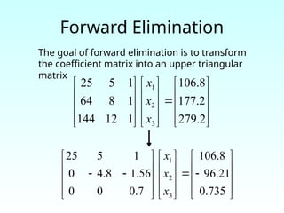
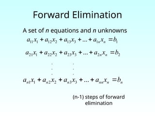
6. Forward Elimination
A set of n equations and n unknowns
1
1
3
13
2
12
1
11 ... b
x
a
x
a
x
a
x
a n
n 




2
2
3
23
2
22
1
21 ... b
x
a
x
a
x
a
x
a n
n 




n
n
nn
n
n
n b
x
a
x
a
x
a
x
a 



 ...
3
3
2
2
1
1
. .
. .
. .
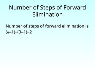
(n-1) steps of forward
elimination

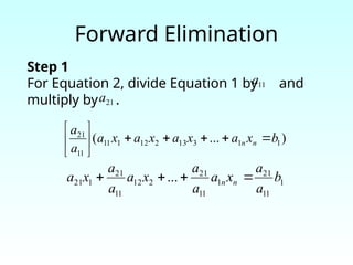
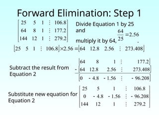
7. Forward Elimination
Step 1
For Equation 2, divide Equation 1 by and
multiply by .
)
...
( 1
1
3
13
2
12
1
11
11
21
b
x
a
x
a
x
a
x
a
a
a
n
n 










1
11
21
1
11
21
2
12
11
21
1
21 ... b
a
a
x
a
a
a
x
a
a
a
x
a n
n 



11
a
21
a

8. Forward Elimination
1
11
21
1
11
21
2
12
11
21
1
21 ... b
a
a
x
a
a
a
x
a
a
a
x
a n
n 



1
11
21
2
1
11
21
2
2
12
11
21
22 ... b
a
a
b
x
a
a
a
a
x
a
a
a
a n
n
n 





















'
2
'
2
2
'
22 ... b
x
a
x
a n
n 


2
2
3
23
2
22
1
21 ... b
x
a
x
a
x
a
x
a n
n 




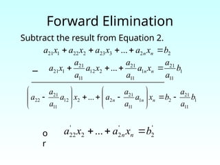
Subtract the result from Equation 2.
−
_________________________________________________
o
r

9. Forward Elimination
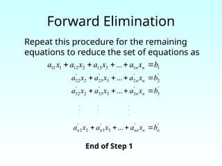
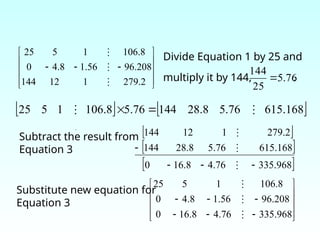
Repeat this procedure for the remaining
equations to reduce the set of equations as
1
1
3
13
2
12
1
11 ... b
x
a
x
a
x
a
x
a n
n 




'
2
'
2
3
'
23
2
'
22 ... b
x
a
x
a
x
a n
n 



'
3
'
3
3
'
33
2
'
32 ... b
x
a
x
a
x
a n
n 



'
'
3
'
3
2
'
2 ... n
n
nn
n
n b
x
a
x
a
x
a 



. . .
. . .
. . .
End of Step 1

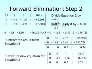
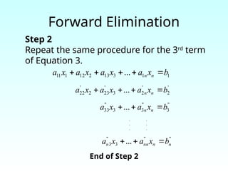
10. Step 2
Repeat the same procedure for the 3rd
term
of Equation 3.
Forward Elimination
1
1
3
13
2
12
1
11 ... b
x
a
x
a
x
a
x
a n
n 




'
2
'
2
3
'
23
2
'
22 ... b
x
a
x
a
x
a n
n 



"
3
"
3
3
"
33 ... b
x
a
x
a n
n 


"
"
3
"
3 ... n
n
nn
n b
x
a
x
a 


. .
. .
. .
End of Step 2

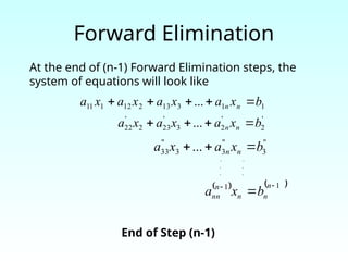
11. Forward Elimination
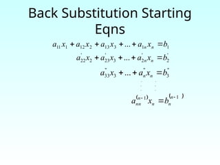
At the end of (n-1) Forward Elimination steps, the
system of equations will look like
'
2
'
2
3
'
23
2
'
22 ... b
x
a
x
a
x
a n
n 



"
3
"
3
3
"
33 ... b
x
a
x
a n
n 


   
1
1 


n
n
n
n
nn b
x
a
. .
. .
. .
1
1
3
13
2
12
1
11 ... b
x
a
x
a
x
a
x
a n
n 




End of Step (n-1)

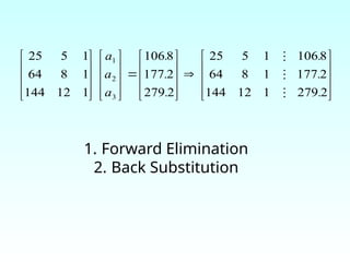
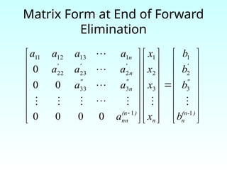
12. Matrix Form at End of Forward
Elimination

















































 )
(n-
n
"
'
n
)
(n
nn
"
n
"
'
n
'
'
n
b
b
b
b
x
x
x
x
a
a
a
a
a
a
a
a
a
a
1
3
2
1
3
2
1
1
3
33
2
23
22
1
13
12
11
0
0
0
0
0
0
0











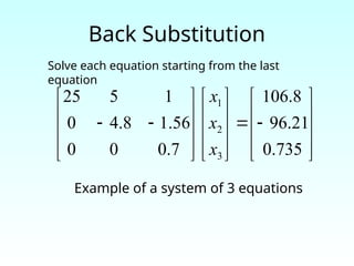
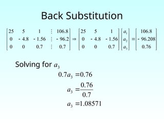
13. Back Substitution
Solve each equation starting from the last
equation
Example of a system of 3 equations


































735
.
0
21
.
96
8
.
106
7
.
0
0
0
56
.
1
8
.
4
0
1
5
25
3
2
1
x
x
x

14. Back Substitution Starting
Eqns
'
2
'
2
3
'
23
2
'
22 ... b
x
a
x
a
x
a n
n 



"
3
"
3
"
33 ... b
x
a
x
a n
n 


   
1
1 


n
n
n
n
nn b
x
a
. .
. .
. .
1
1
3
13
2
12
1
11 ... b
x
a
x
a
x
a
x
a n
n 





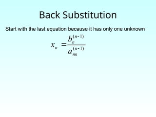
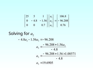
15. Back Substitution
Start with the last equation because it has only one unknown
)
1
(
)
1
(


 n
nn
n
n
n
a
b
x

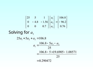
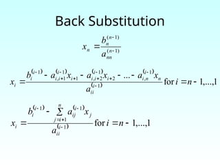
16. Back Substitution
   
  1
,...,
1
for
1
1
1
1




 




n
i
a
x
a
b
x i
ii
n
i
j
j
i
ij
i
i
i
)
1
(
)
1
(


 n
nn
n
n
n
a
b
x
       
  1
,...,
1
for
...
1
1
,
2
1
2
,
1
1
1
,
1






 








n
i
a
x
a
x
a
x
a
b
x i
ii
n
i
n
i
i
i
i
i
i
i
i
i
i
i
i

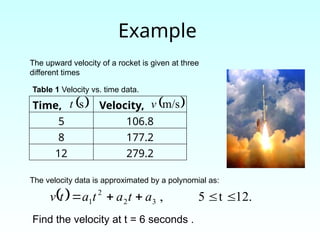
17. Example
The upward velocity of a rocket is given at three
different times
Time, Velocity,
5 106.8
8 177.2
12 279.2
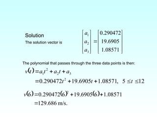
The velocity data is approximated by a polynomial as:
  12.
t
5
,
3
2
2
1 



 a
t
a
t
a
t
v
Find the velocity at t = 6 seconds .
 
s
t  
m/s
v
Table 1 Velocity vs. time data.

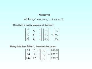
18. Assume
  12.
t
5
,
a
t
a
t
a
t
v 



 3
2
2
1































3
2
1
3
2
3
2
2
2
1
2
1
1
1
1
v
v
v
a
a
a
t
t
t
t
t
t
3
2
1
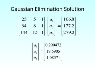
Results in a matrix template of the form:
Using data from Table 1, the matrix becomes:































2
.
279
2
.
177
8
.
106
1
12
144
1
8
64
1
5
25
3
2
1
a
a
a

19. 









































2
279
1
12
144
2
177
1
8
64
8
106
1
5
25
2
279
2
177
8
106
1
12
144
1
8
64
1
5
25
3
2
1
.
.
.
.
.
.
a
a
a



1. Forward Elimination
2. Back Substitution

20. Forward Elimination

21. Number of Steps of Forward
Elimination
Number of steps of forward elimination is
(n-1)=(3-1)=2

22. Divide Equation 1 by 25
and
multiply it by 64, .
Forward Elimination: Step 1
.
   
408
.
273
56
.
2
8
.
12
64
56
.
2
8
.
106
1
5
25 
 

 
 
 
208
.
96
56
.
1
8
.
4
0
408
.
273
56
.
2
8
.
12
64
177.2
1
8
64

















2
.
279
1
12
144
2
.
177
1
8
64
8
.
106
1
5
25
















2
.
279
1
12
144
208
.
96
56
.
1
8
.
4
0
8
.
106
1
5
25



56
.
2
25
64

Subtract the result from
Equation 2
Substitute new equation for
Equation 2

23. .
   
168
.
615
76
.
5
8
.
28
144
76
.
5
8
.
106
1
5
25 
 














2
.
279
1
12
144
208
.
96
56
.
1
8
.
4
0
8
.
106
1
5
25



 
 
 
968
.
335
76
.
4
8
.
16
0
168
.
615
76
.
5
8
.
28
144
279.2
1
12
144























968
.
335
76
.
4
8
.
16
0
208
.
96
56
.
1
8
.
4
0
8
.
106
1
5
25



Divide Equation 1 by 25 and
multiply it by 144, .
76
.
5
25
144

Subtract the result from
Equation 3
Substitute new equation for
Equation 3

24. Forward Elimination: Step 2
   
728
.
336
46
.
5
8
.
16
0
5
.
3
208
.
96
56
.
1
8
.
4
0 






 

















968
.
335
76
.
4
8
.
16
0
208
.
96
56
.
1
8
.
4
0
8
.
106
1
5
25



 
 
 
.76
0
7
.
0
0
0
728
.
336
46
.
5
16.8
0
335.968
76
.
4
16.8
0






















76
.
0
7
.
0
0
0
208
.
96
56
.
1
8
.
4
0
8
.
106
1
5
25



Divide Equation 2 by
4.8
−
and multiply it by 16.8,
−
.
5
.
3
8
.
4
8
.
16



Subtract the result from
Equation 3
Substitute new equation for
Equation 3

25. Back Substitution

26. Back Substitution
















































76
.
0
208
.
96
8
.
106
7
.
0
0
0
56
.
1
8
.
4
0
1
5
25
7
.
0
7
.
0
0
0
2
.
96
56
.
1
8
.
4
0
8
.
106
1
5
25
3
2
1
a
a
a



08571
.
1
7
.
0
76
.
0
76
.
0
7
.
0
3
3
3



a
a
a
Solving for a3

27. Solving for a2
6905
19.
4.8
1.08571
1.56
96.208
8
.
4
56
.
1
208
.
96
208
.
96
56
.
1
8
.
4
2
2
3
2
3
2














a
a
a
a
a
a


































76
.
0
208
.
96
8
.
106
7
.
0
0
0
56
.
1
8
.
4
0
1
5
25
3
2
1
a
a
a

28. Solving for a1
290472
.
0
25
08571
.
1
6905
.
19
5
8
.
106
25
5
8
.
106
8
.
106
5
25
3
2
1
3
2
1











a
a
a
a
a
a


































76
.
0
2
.
96
8
.
106
7
.
0
0
0
56
.
1
8
.
4
0
1
5
25
3
2
1
a
a
a

29. Gaussian Elimination Solution































2
279
2
177
8
106
1
12
144
1
8
64
1
5
25
3
2
1
.
.
.
a
a
a





















08571
.
1
6905
.
19
290472
.
0
3
2
1
a
a
a

30. Solution
The solution vector is





















08571
.
1
6905
.
19
290472
.
0
3
2
1
a
a
a
The polynomial that passes through the three data points is then:
 
12
5
,
08571
.
1
6905
.
19
290472
.
0 2
3
2
2
1








t
t
t
a
t
a
t
a
t
v
     
.
m/s
686
.
129
08571
.
1
6
6905
.
19
6
290472
.
0
6
2




v