Downloaded 362 times


![Augmented matrix:
][3
2
1
321
3333231
2232221
1131211
bA
b
b
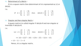
b
b
aaaa
aaaa
aaaa
aaaa
mmnmmm
n
n
n
A
aaaa
aaaa
aaaa
aaaa
mnmmm
n
n
n
321
3333231
2232221
1131211
Coefficient matrix:](https://image.slidesharecdn.com/systemoflinearequationsandmatrices-150508143106-lva1-app6891/85/system-linear-equations-and-matrices-22-320.jpg)
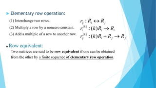
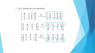
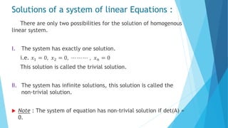

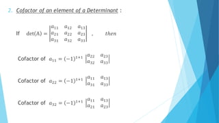
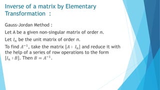
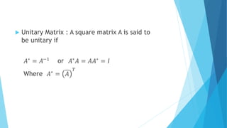


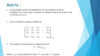
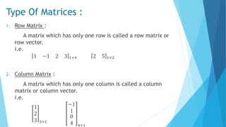
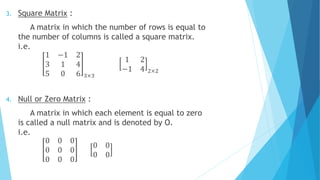
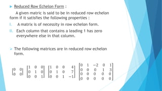
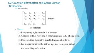
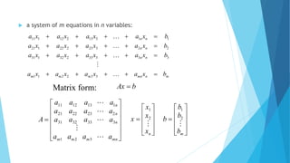
The document provides a comprehensive overview of matrices and systems of linear equations, detailing various types of matrices such as row, column, square, and diagonal matrices, along with their properties and operations. It discusses methods for solving systems of linear equations, including Gaussian elimination and Gauss-Jordan elimination, as well as the concepts of equivalent matrices, row echelon forms, and reduced row echelon forms. Furthermore, it explains the conditions for singular and non-singular matrices and lays out the framework for representing linear equations in matrix form.


![43040989[1]](https://cdn.slidesharecdn.com/ss_thumbnails/430409891-100920031026-phpapp02-thumbnail.jpg?width=640&height=640&fit=bounds)


