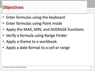
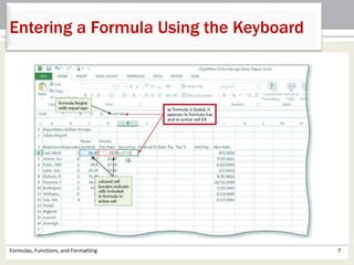
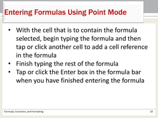
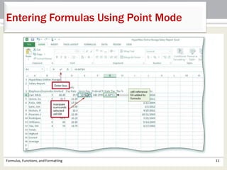
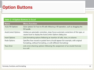
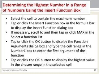
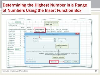
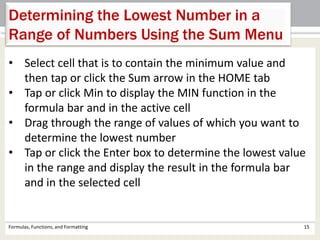
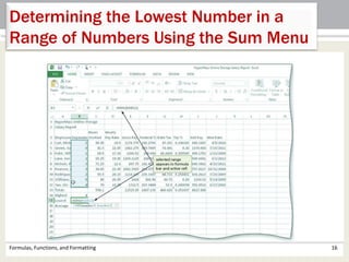
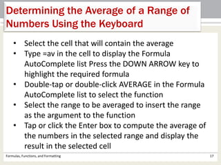
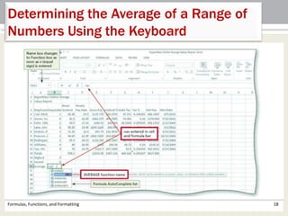
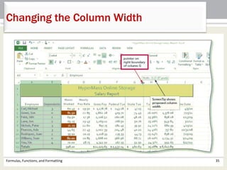
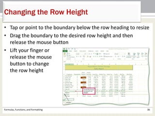
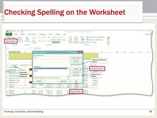
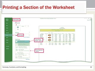
This document provides objectives and instructions for Chapter 2 of a Microsoft Excel 2013 textbook. The chapter covers entering formulas using the keyboard or point mode, applying functions like MAX, MIN and AVERAGE, verifying formulas, formatting worksheets by applying themes, date formats and conditional formatting, adjusting column width and row height, checking spelling, changing print settings and margins, and printing sections of a worksheet.
اكسيل كارت الاستخدام السريع لحساب الارباح و الوارد و المنصرف لاصحاب الاعمال ...Ahmed Farahat
رَبِّ اغْفِرْ لِي وَلِوَالِدَيَّ وَلِمَن دَخَلَ بَيْتِيَ مُؤْمِنًا وَلِلْمُؤْمِنِينَ وَالْمُؤْمِنَاتِ وَلَا تَزِدِ الظَّالِمِينَ إِلَّا تَبَارًا
مع تحيات م/ احمد جاد الله فرحات
العمل الحر,
الدعايه و التصميم,
فن الاعلان,
العمل من المنزل ,
Adobe Illustrator,
الدعاية و الاعلان,
الجرفيكس ,
العمل الحر,
مشاريع قوت اليوم ,
العمل من المنزل ,
ربح المال ,
العمل الحر,
التدقيق اللغوي ,
الترجمة ,
تعليم اللغات ,
كتابة المحتوي,
Describe the Excel worksheet. Enter text and numbers and use the Sum button to sum a range of cells. Copy the contents of a cell to a range of cells using the fi ll handle. Apply cell styles and format cells in a worksheet. Create an embedded chart. Change a worksheet name and worksheet tab color. Change document properties and print preview and a worksheet. Use AutoCalculate to display statistics.
Research students find it difficult to edit Word Documents since they would have not explored all avenues of systematic editing features in this desk top publishing. The slides showed herein describe systematic methodology to create a thesis template for presenting Project thesis, research thesis etc., The contents include, page setup, setting up headings, sub headings, sub-sub headings, creating tables and hyperlinking table labels, creating labels for figures and hyperlinking, automatic generation of listing of Contents, list of Figures, Tables, and more interestingly creating reference listing (bibliography) and hyperlinking with citation in the text, and overall reference management. The merging of smaller documents to create a master document in Word is another useful hint for managing Word documents with large number of pages. Students who may not like to edit thesis using Latex can comfortably make use of this slide share.
2. • Enter formulas using the keyboard
• Enter formulas using Point mode
• Apply the MAX, MIN, and AVERAGE functions
• Verify a formula using Range Finder
• Apply a theme to a workbook
• Apply a date format to a cell or range
Objectives
Formulas, Functions, and Formatting 2
3. • Add conditional formatting to cells
• Change column width and row height
• Check the spelling on a worksheet
• Change margins and headers in Page Layout view
• Preview and print versions and sections of a
worksheet
Formulas, Functions, and Formatting 3
Objectives
5. • Enter formulas in the worksheet
• Enter functions in the worksheet
• Verify formulas in the worksheet
• Format the worksheet
• Check spelling
• Print the worksheet
Formulas, Functions, and Formatting 5
Roadmap
6. Formulas, Functions, and Formatting 6
Entering a Formula Using the Keyboard
• With the cell to contain the formula selected,
type the formula in the cell to display the
formula in the formula bar and in the current
cell and to display colored borders around the
cells referenced in the formula
• Press the right arrow key to complete the
arithmetic operation indicated by the formula,
to display the result in the worksheet, and to
select the cell to the right
10. Formulas, Functions, and Formatting 10
Entering Formulas Using Point Mode
• With the cell that is to contain the formula
selected, begin typing the formula and then
tap or click another cell to add a cell reference
in the formula
• Finish typing the rest of the formula
• Tap or click the Enter box in the formula bar
when you have finished entering the formula
13. Formulas, Functions, and Formatting 13
Determining the Highest Number in a Range
of Numbers Using the Insert Function Box
• Select the cell to contain the maximum number
• Tap or click the Insert Function box in the formula bar
to display the Insert Function dialog box
• If necessary, scroll to and then tap or click MAX in the
Select a function list
• Tap or click the OK button to display the Function
Arguments dialog box and type the cell range in the
Number1 box to enter the first argument of the
function
• Tap or click the OK button to display the highest value
in the chosen range in the selected cell
14. Formulas, Functions, and Formatting 14
Determining the Highest Number in a Range
of Numbers Using the Insert Function Box
15. Formulas, Functions, and Formatting 15
Determining the Lowest Number in a
Range of Numbers Using the Sum Menu
• Select cell that is to contain the minimum value and
then tap or click the Sum arrow in the HOME tab
• Tap or click Min to display the MIN function in the
formula bar and in the active cell
• Drag through the range of values of which you want to
determine the lowest number
• Tap or click the Enter box to determine the lowest value
in the range and display the result in the formula bar
and in the selected cell
16. Formulas, Functions, and Formatting 16
Determining the Lowest Number in a
Range of Numbers Using the Sum Menu
17. Formulas, Functions, and Formatting 17
Determining the Average of a Range of
Numbers Using the Keyboard
• Select the cell that will contain the average
• Type =av in the cell to display the Formula
AutoComplete list Press the DOWN ARROW key to
highlight the required formula
• Double-tap or double-click AVERAGE in the Formula
AutoComplete list to select the function
• Select the range to be averaged to insert the range
as the argument to the function
• Tap or click the Enter box to compute the average of
the numbers in the selected range and display the
result in the selected cell
18. Formulas, Functions, and Formatting 18
Determining the Average of a Range of
Numbers Using the Keyboard
19. Formulas, Functions, and Formatting 19
Verifying a Formula using Range Finder
• Double-tap or double-click a cell to activate Range
Finder
• Press the ESC
key to quit
Range Finder
and then tap
or click
anywhere in
the worksheet
to deselect the
current cell
21. Formulas, Functions, and Formatting 21
Changing the Workbook Theme
• Tap or click the Themes button on the PAGE LAYOUT tab
to display the Themes gallery
• Tap or click the
desired theme
in the Themes
gallery to change
the workbook
theme
22. • Select the range to color and then tap or click the Fill
Color arrow on the HOME tab to display the Fill Color
gallery
• Tap or click a color to select it and change the
background color of the range of cells
• Tap or click the Borders arrow on the HOME tab to
display the Borders gallery
• Tap or click a border in the Borders gallery to select it
and display a border around the selected range
Formulas, Functions, and Formatting 22
Changing the Background Color and Applying a
Box Border to the Worksheet Title and Subtitle
23. Formulas, Functions, and Formatting 23
Changing the Background Color and Applying a
Box Border to the Worksheet Title and Subtitle
24. Formulas, Functions, and Formatting 24
Formatting Dates and Centering Data in
Cells
• Select the range to contain the new date format
• Tap or click the Format Cells: Number Format Dialog Box Launcher
in the HOME tab to display the dialog box
• If necessary, tap or click the NUMBER tab and tap or click Date in
the Category list, and then tap or click a date type to choose the
format for the selected range
• Tap or click the NUMBER tab and then tap or click Date in the
Category list to choose the format for the selected range
• Tap or click the OK button to format the dates in the current
column using the selected date format style
• Select the range to be centered and then tap or click the Center
button on the HOME tab to center the data in the selected range
26. • Select the range to contain the accounting number
format
• While holding down the CTRL key, select the nonadjacent
ranges and cells
• Tap or click the ‘Accounting Number Format’ button on
the HOME tab to apply the accounting number format to
the selected nonadjacent ranges
• Tap or click the Comma Style button on the HOME tab to
assign the Comma style format to the selected range
Formulas, Functions, and Formatting 26
Applying an Accounting Number Format and
Comma Style Format Using the Ribbon
27. Formulas, Functions, and Formatting 27
Applying an Accounting Number Format and
Comma Style Format Using the Ribbon
28. Formulas, Functions, and Formatting 28
Applying a Currency Style Format with a Floating
Dollar Sign Using the Format Cells Dialog Box
• Select the range to format and then tap or click the
Number Format Dialog Box Launcher in the HOME tab
to display the Format Cells dialog box
• If necessary, tap or click the NUMBER tab to display the
Number sheet
• Tap or click Currency in the Category list to select the
necessary number format category and then tap or click
a style in the Negative numbers list to select the desired
currency format
• Tap or click the OK button to assign the currency style
format to the selected ranges
29. Formulas, Functions, and Formatting 29
Applying an Currency Style Format with a Floating
Dollar Sign Using the Format Cells Dialog Box
30. • Select the range to format
• Tap or click the Percent Style button in the HOME tab to
display the numbers in the selected range as a rounded
whole percent
• Tap or click the
Increase Decimal
button in the HOME
tab two times to
display the numbers
in the selected range
with two decimal
places
Formulas, Functions, and Formatting 30
Applying Percent Style Format and Using
the Increase Decimal Button
31. • Select the range to which you wish to apply
conditional formatting
• Tap or click the Conditional Formatting button on the
HOME tab to display the Conditional Formatting list
• Tap or click New Rule in the Conditional Formatting
list to display the New Formatting Rule dialog box
• Tap or click the desired rule type in the Select a Rule
Type area
• Select and type the desired values in the Edit the Rule
Description area
Formulas, Functions, and Formatting 31
Applying Conditional Formatting
34. • Drag through column headings to select the columns
• Tap or point to the boundary on the rightmost column
heading to cause the pointer to become a split double arrow
• Double-tap or double-click the right boundary of the column
to change the width of the selected columns to best fit
• To resize a column by dragging, point to the boundary of the
right side of the column heading. When the mouse pointer
changes to a split double arrow, drag to the desired width,
and then Lift your finger or release the mouse button to
change the column widths
Formulas, Functions, and Formatting 34
Changing the Column Width
36. • Tap or point to the boundary below the row heading to resize
• Drag the boundary to the desired row height and then
release the mouse button
• Lift your finger or
release the mouse
button to change
the row height
Formulas, Functions, and Formatting 36
Changing the Row Height
37. • Tap or click cell A1 so that the spell checker begins at
the beginning of the worksheet
• Tap or click the Spelling button on the REVIEW tab to
run the spell checker and display the misspelled
words in the Spelling dialog box
• Apply the desired action to each misspelled word
• When the spell checker is finished, Tap or click the
Close button
Formulas, Functions, and Formatting 37
Checking Spelling on the Worksheet
39. • Tap or click the Page Layout button on the status bar to
view the worksheet in Page Layout view
• Tap or click the Adjust Margins button on the PAGE
LAYOUT tab to display the Margins gallery
• Tap or click the desired margin style to change the
worksheet margins to the selected style
• Tap or click above cell A1 in the center area of the Header
area
• Type the desired worksheet header, and then press the
ENTER key
Formulas, Functions, and Formatting 39
Changing the Worksheet’s Margins, Header,
and Orientation in Page Layout View
40. Formulas, Functions, and Formatting 40
Changing the Worksheet’s margins, header,
and Orientation in Page Layout View
41. • Tap or click the ‘Change Page Orientation’ button on the
PAGE LAYOUT tab to display the Change Page Orientation
gallery
• Tap or click the
desired orientation
in the Orientation
gallery to change
the worksheet’s
orientation
Formulas, Functions, and Formatting 41
Changing the Worksheet’s margins, header,
and Orientation in Page Layout View
42. Formulas, Functions, and Formatting 42
Printing a Section of the Worksheet
• Select the range to print
• Tap or click FILE on the ribbon to open Backstage view
• Tap or click the Print tab to display the Print gallery
• Tap or click ‘Print Active Sheets’ in the Settings area on
the PRINT tab to display a list of printing options
• Tap or click Print Selection to print the selected range
• Tap or click the Print button in the Print gallery to print
the selected range of the worksheet
• Tap or click the Normal button on the status bar to return
to Normal view
44. Formulas, Functions, and Formatting 44
Displaying the Formulas in the Worksheet
and Fitting the Printout on One Page
• Press CTRL+ACCENT MARK (`) to display the worksheet with
formulas
• Tap or click the Page Setup Dialog Box Launcher on the PAGE
LAYOUT tab to display the Page Setup dialog box
• If necessary, tap or click the desired Orientation in the Page sheet
to select it
• If necessary, tap or click Fit to in the Scaling area to select it
• Tap or click the Print button to print the formulas in the worksheet
on one page. If necessary, in the Backstage view, select the Print
Active Sheets option in the Settings area of the Print gallery
• When Excel displays the Backstage view, tap or click the Print
button to print the worksheet
• After viewing and printing the formulas version, press
CTRL+ACCENT MARK (`) to display the values version
45. Formulas, Functions, and Formatting 45
Displaying the Formulas in the Worksheet
and Fitting the Printout on One Page
46. Chapter Summary
Formulas, Functions, and Formatting 46
• Enter formulas using the keyboard
• Enter formulas using Point mode
• Apply the MAX, MIN, and AVERAGE functions
• Verify a formula using Range Finder
• Apply a theme to a workbook
• Apply a date format to a cell or range
47. Chapter Summary
Formulas, Functions, and Formatting 47
• Add conditional formatting to cells
• Change column width and row height
• Check the spelling on a worksheet
• Change margins and headers in Page Layout view
• Preview and print versions and sections of a worksheet